 Overhead 1
Thermochronology
Part I: Ar-Ar Geo-/Thermochronology
(accompanying explanations, © Priv.-Doz. Dr. Jörg A. Pfänder)
Textbooks you may use in Part 1:
- Ian McDougall & Mark T. Harrison: Geochronology and Thermochronology by the 40Ar/39Ar Method. Oxford Universitys Press
- Jean Braun, Peter van der Beek, Geoffrey Batt: Quantitative Thermochronology. Cambridge University Press
 Overhead 2
The basis of the Ar-Ar radioisotope dating technique is the K-Ar dating technique, which itself is based on the radioactive decay of 40K to stable 40Ar. This decay was postulated from nuclear physics considerations and 40Ar abundances in 1937 by Carl Friedrich von Weizsäcker. Aldrich and Nier proofed in 1948 that 40Ar indeed is a decay product of 40K. They inferred this from much higher 40Ar/36Ar isotope ratios observed in the K-rich mineral Langbeinite than in the present day atmosphere. Note in this context, that our atmosphere contains as much as ~0.9% of Argon with a 40Ar/36Ar isotope abundance ratio of ~298.
Overhead 3
This is the first page of the publication of Aldrich and Nier from 1948. Note, at least, the marked text. As you can see, 40K decays not only to stable 40Ar, but also to stable 40Ca.
Overhead 4
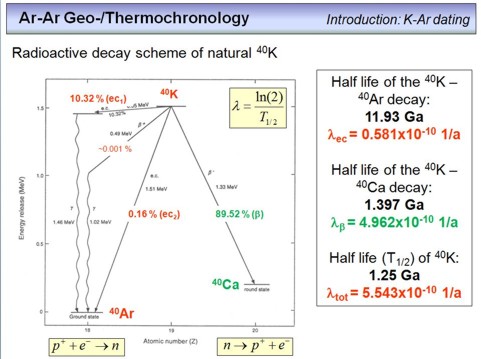 This overhead is quite important as it shows the decay schemes of 40K, that not only produces stable 40Ar, but also stable 40Ca. It is very important to realize that the 40K in a mineral produces 40Ar and 40Ca at different production rates. We term this a branched decay.
From the energy term scheme shown on the left, we can derive several important issues. First, ~10.32% of the 40K in a mineral decays by an electron capture decay to excited 40Ar. This excited 40Ar is unstable and continues to decay very quickly to stable 40Ar in its ground state, by emitting γ-rays with an energy of 1.46 MeV. Note that ~0.16% of the 40K decays directly to stable 40Ar in its ground state, and that a very tiny amount of 40K (~0.001%) decays via °+-emission to an exited 40Ar and from there also to stable 40Ar in its ground state. Overall, if we sum this up, we can see that:
This overhead is quite important as it shows the decay schemes of 40K, that not only produces stable 40Ar, but also stable 40Ca. It is very important to realize that the 40K in a mineral produces 40Ar and 40Ca at different production rates. We term this a branched decay.
From the energy term scheme shown on the left, we can derive several important issues. First, ~10.32% of the 40K in a mineral decays by an electron capture decay to excited 40Ar. This excited 40Ar is unstable and continues to decay very quickly to stable 40Ar in its ground state, by emitting γ-rays with an energy of 1.46 MeV. Note that ~0.16% of the 40K decays directly to stable 40Ar in its ground state, and that a very tiny amount of 40K (~0.001%) decays via °+-emission to an exited 40Ar and from there also to stable 40Ar in its ground state. Overall, if we sum this up, we can see that:
32% + 0.16% + 0.001% = 10.48%
of the 40K in a mineral decays to stable 40Ar. The decay rate of this process, i.e. the likelyhood that 40K disappears to end up as 40Ar is λec = 0.581 x 10⁻¹⁰ per year (1/a), where λec is the decay constant (corresponding to a half-life (T1/2) of 11.93 billion years, i.e. 11.93 Ga, see the formula in the overhead).
The second decay is the decay of 40K to stable 40Ca, with a decay constant of 4.962 x 10⁻¹⁰ 1/a (T1/2= 1.397 Ga). This means that 89.52% of the 40K in a mineral decays not to 40Ar, but to 40Ca, i.e. is "lost" for our purposes (but, K is an abundant element, so we don't care, this is not a problem).
Taking all decays together, i.e. summing up all the decay constants, we can see that the rate at which 40K disappears is 5.543 x 10⁻¹⁰ corresponding to a half life of 1.25 Ga. This means that 40K is much faster consumed than 40Ar is build, a circumstance that we need to consider later when we derive the age equations for the K-Ar and Ar-Ar geochronometers.
Overhead 5
This overhead basically shows the same as what we have seen in overhead 4, but now in the chart of nuclides. Think about it, and try to understand the nuclear reactions that are involved in the mentioned decay schemes. Note, that n denotes a neutron, p+ a proton, e- an electron, and e+ a positron.
Overhead 6
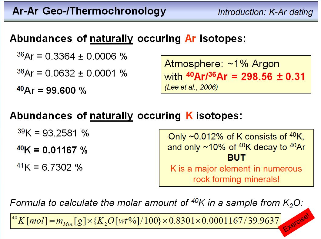 Doing geochronology requires knowledge about the isotope abundances of the elements involved. This is shown here. Note that the parent isotope of the K-Ar and Ar-Ar techniques, 40K, is not very abundant in nature, but as K is a major element in many rock forming minerals this is of minor disadvantage.
Among the three stable Ar-isotopes, the daughter isotope of interest, 40Ar, is the by far most abundant one, and its ratio over 36Ar in the Argon that is part of our atmosphere is 298.56±0.31. Note that the air we breath contains ~0.9 vol% Ar. This atmospheric 40Ar/36Ar ratio is of great importance and you should keep this in mind.
The formula on the bottom of this overhead allows to calculate the molar amount of 40K in a rock or mineral from its K2O-content. The constant 0.8301 transfers the wt% K2O into wt% K, the constant 0.0001167 is the abundance of the 40K-isotope, and the constant 39.9637 is the atomic mass of 40K (a bit less than 40 due to the mass defect, that was transformed into energy according to E=mc2). If you need to refresh your knowledge about moles,
watch this!
Overhead 7
This overhead gives an overview about the phases (minerals and whole-rock fragments) that can be dated by the K-Ar and Ar-Ar technique. Principally any type of rock or mineral that contains sufficient K is suitable. The diagram in the lower part shows the age range coverd by these methods, and this age range depends primarily on the K-content, the more, the better. The photograph on the upper right shows a sample holder how it is used in our lab
(Argonlab Freiberg, ALF)
It is made of oxygen-free copper, has a diameter of 50 mm, and holes with a diameter of 3 mm each. In the holes you can see ~2-3 mg of mineral separates (dark: biotite, bright: muscovite or k-feldspar), ready for laser heating and measurement.
Overhead 8
 According to the radioactive decay law (see here in
german
or in
english),
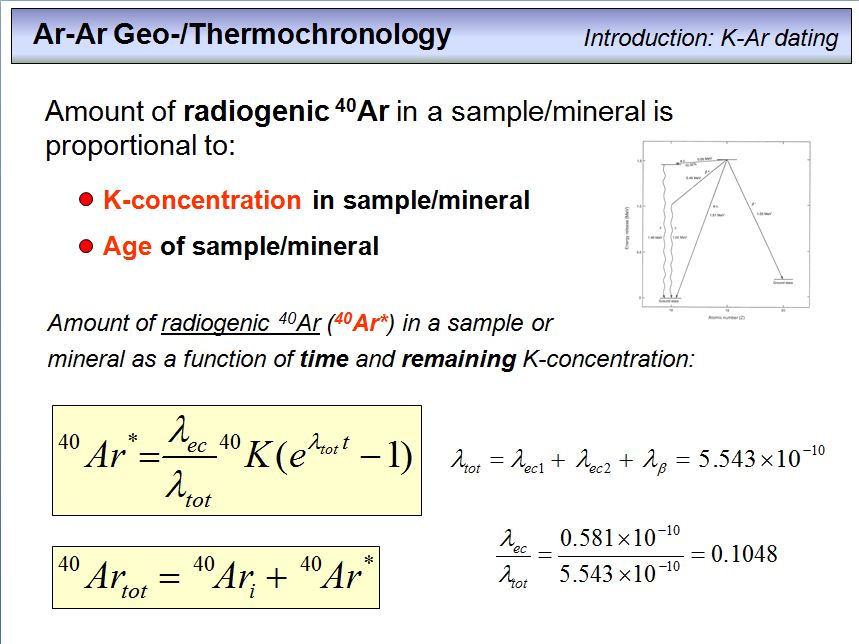
the amount of radiogenic 40Ar that accumulates in a rock or mineral over time is a function of its initial K-content (40K) and time (that means age of this rock or mineral). The more K is in a mineral, and the older this mineral is, the more radiogenic, or decay produced, 40Ar will accumulate in it (note that we will term 40Ar that is produced from the decay of 40K as radiogenic 40Ar in the following, and use the abbreviation 40Ar* for it).
According to the radioactive decay law (see here in
german
or in
english),
the amount of radiogenic 40Ar that accumulates in a rock or mineral over time is a function of its initial K-content (40K) and time (that means age of this rock or mineral). The more K is in a mineral, and the older this mineral is, the more radiogenic, or decay produced, 40Ar will accumulate in it (note that we will term 40Ar that is produced from the decay of 40K as radiogenic 40Ar in the following, and use the abbreviation 40Ar* for it).
The first formula in the yellow box is the formula to calculate the number (i.e. moles) of radiogenic 40Ar atoms (40Ar*) that were produced in a rock or mineral after a specific time (t) and for a given K-concentration, i.e. a given number of 40K atoms (moles). NOTE that the 40K content used in this formula is the amount of 40K that has left after time t has elapsed. This means that this formula enables us to calculate the amount of 40Ar* in a rock or mineral of age t from its present day 40K content (where that latter can be calculated from the K2O-content as measured by the electron probe and using the natural K-isotope abundances, see above). Vice versa we can calculate the age of a rock or mineral if we know its present-day abundance of 40K and 40Ar* (note that necessarily the sum of 40Ar* and 40K in a rock or mineral today provides the amount of 40K that was present in the rock or mineral at the time of its formation). Be aware that if a rock or mineral forms, it is not necessarily free of argon. That means that upon its growth a mineral my incorporate argon with a distinct isotope composition in its lattice. We call this argon initial argon, and abbreviate it as Ari. Consequently, the total amount of 40Ar in a rock or mineral that we can measure today is the sum of 40Ari and 40Ar*, as denoted in the second yellow box.
Taking all these information, and the information provided in overhead 6, you now should be able to solve the following
exercise (moles).
Overhead 9
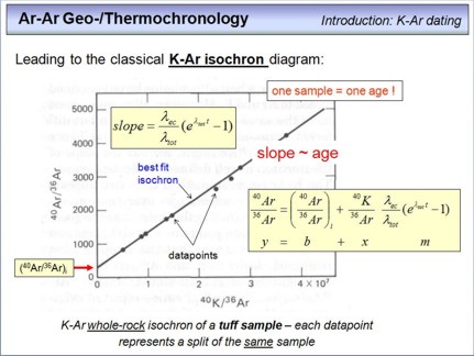 All information outlined above brings us to the classical isochron diagram, which is valid for any radioisotope chronometer (Sm-Nd, U-Pb, Th-Pb, Lu-Hf, Rb-Sr, Re-Os, K-Ar).
In this diagram, the parent isotope is denoted on the x-axis, and the daughter isotope on the y-axis. But as you can see, not the absolute amounts (moles) are denoted here for 40K and 40Ar that have been measured in a rock or mineral on a mass spectrometer, but isotope ratios. This has simply practical reasons, namely that isotope ratios can be measured much more precise than absolute amounts, and 'normalizing' both quantities to the same 'reference' isotope (here 36Ar) doesn't change anything with respect to the result. Therefore, the lower right equation is the result of combining the two equations from the previous overhead, and then dividing each term by 36Ar (note that any isotope abundance is in mole). The equation is the isochron equation for the K-Ar dating technique and is mathematically a linear function with the slope m and the y-axis intercept b in terms of x (40K/36Ar) and y (40Ar/36Ar). The slope itself is, as you can see from the upper left equation, a function of the age of the rock(s) or mineral(s).
What is shown in detail here? The black points are datapoints, each point represents the 40K/36Ar and 40Ar/36Ar ratio of a small sample fragment from a volcanic tuff layer (i.e., nine fragments have been taken from this tuff sample). All nine datapoints plot along a straight line, this is the isochron. From this linear correlation the slope can be calculated, and from this slope the age of the sample. The initial 40Ar/36Ar can also be calculated, and this is the isotope composition of the argon that was incorporated in all analysed fragments during their formation. See the following
exercise (K-Ar age).
Overhead 10
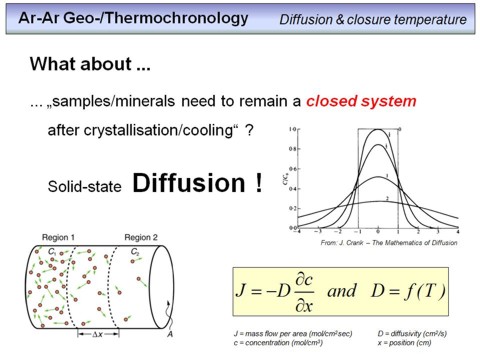
We have seen that if we know the amount of K and Ar in a sample, and the isotope abundances of these elements, we can calculate a radioisotopic K-Ar age for this sample (or better, for of a cogenetic series of samples). However, to abtain a real geologically significant age, some requirements have to be fulfilled, and these requirements are summarized on this overhead. The last point is the most critical one, and we will consider this in more detail in the following. It concerns the fact that an age is only correct, if a rock or mineral remained a closed system after crystallisation. That is, after formation, a mineral must not gain or loose any of its potassium or argon, otherwise the resulting age will be wrong, either to low or too high. As this condition is often not fulfilled in real samples, we have briefly to go into diffusion processes, as solid-state diffusion is the mechanism that corroborates K-Ar and Ar-Ar ages, typically because of post-formation argon loss.
Overhead 11
 Diffusion
is the movement of atoms or ions within a solid phase (isotropic or anisotropic), from outside into a solid phase, or from inside out of a solid phase.
Watch this
to get an impression on how argon atoms diffuse from atmosphere into a solid phase.
Diffusion
is the movement of atoms or ions within a solid phase (isotropic or anisotropic), from outside into a solid phase, or from inside out of a solid phase.
Watch this
to get an impression on how argon atoms diffuse from atmosphere into a solid phase.
Diffusion in a solid phase is schematically shown on this overhead in the lower left. Imagine the red dots are Ar atoms and note that for any temperature higher than 0 Kelvin any atom in a solid phase is oscillating around its lattice position. In the example you can see that the concentration of atoms in the left part of the cylinder is higher than in the right part, this means that we have a concentration gradient from region 1 to region 2. Due to energetic, or better, thermodynamic reasons, the atoms move from the region with the higher concentration to the region with the lower concentration. This process occurs until the concentration is equal in the whole cylinder (corresponding to an energetic minimum, or entropy maximum). The amount of atoms that passes a defined area (A) per time (i.e. the mass flow, unit: mol/cm2) is proportional to the concentration gradient (i.e. the concentration change per distance, unit: mol/cm). The higher the concentration gradient ∂c/∂t, the faster the diffusion. Introducing a proportionality constant, the proportionality transforms into an equation with D being the diffusion coefficient or diffusivity. This euqation is shown in the lower right and was first postulated by
Adolf Fick in 1855. It is the Fick's first law. The most important thing is to know that the diffusion speed, and therefore D is strongly dependent on temperature. The higher the temperature, the faster the diffusion process!
Watch the figure in the upper right. Let the 'box' with the number '0' be an area with a high concentration of argon or anything else. The x-axis marks the position along an arbitrary direction, i.e. left of -1 and right of 1 the concentration is zero, but there is no diffusion barrier. After some time, marked with number '1', the concentration blurs out, the shape of the concentration profile becomes bell shaped. The more time goes, the more the concentration profile blurs out, i.e. the flatter the concentration profile becomes. At time '3', the concentration is nearly equal across the whole distance (note that at position -4 and 4 there are diffusion barriers.
Overhead 12
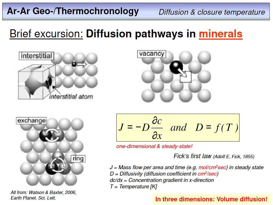 This overhead shows diffusion pathways in minerals (intragranular diffusion). Atoms that are not chemically bond within the lattice can move more easily than such atoms that are chemically bond. We distinguish between interstitial diffusion (an atom moves from an interstitial postion to another interstitial position), vacany diffusion where an atom moves from a vacancy to another vacancy, and exchange diffusion, where an atom moves from a lattice position to another lattice position. Note that such processes are not restricted to uncharged atoms, but ions can also move through a lattice by solid-state diffusion, and the diffusivity depends on the charge and radius of the diffusing species. If diffusion occurs in three dimensions, i.e. the normal case, we call this process volume diffusion. Note that within anisotropic phases, i.e. in most minerals, the diffusivity D is not a vector but a tensor, and its value is direction dependent.
Overhead 13
This overhead shows diffusion pathways in rocks, i.e. between minerals. We call this intergranular diffusion. In this case, atoms such as argon diffuse along the concentration gradient out of a grain into the grain interspace, and from there leave the system or diffuse into another grain, if the concentration within this grain is lower than in the grain interspace. Note that in nature minerals are not ideal solid phases but have lattice defects such as micro- and nano-fractures, subgrain boundaries, point defects etc., and diffusion along such defects is usually faster than pure volume diffusion.
Overhead 14
If diffusion is not in steady state, that means if the mass flow J at a given position is a function of time (i.e. not constant), then the Fick's first law is not applicable as time needs to be considered. Doing so leads to Fick's second law, where the concentration change per time (∂c/∂t) equals the mass flow gradient ∂J/∂x (here in only one direction, namley x). Substituion of J yields the Fick's second law in one dimension.
Overhead 15
This is Fick's second law in three dimensions. It is a differential equation that describes the concentration of any diffusing species in a medium as a function of position (x,y,z) and time (t), if boundary conditions are known.
Overhead 16
This awful equation is a one dimensional analytical solution of Fick's second law for a plane sheet geometry. This means that diffusion is considered in only one direction in a plane sheet with infinite lateral extension, with a diffusion direction perpendicular to the upper and lower boundary (marked with 2r in the figure on the right). This equation demonstrates that solving Fick's second law requires assumptions about the geometry of the phase for which diffusion is considerd. With regard to K-Ar and Ar-Ar geochronology assuming a plane sheet geometry is justified, for examle, for micas such as biotite or muscovite. In such phases, argon diffusion will predominantly occur along the crystallographic c-axis.
Overhead 17
This equation is a solution of Fick's second law for a spherical geometry and hence in sperical coordinates. It is similar to the solution before, with only a single variable, the position R within the sphere.
Overhead 18
The need to establish analytical solutions of the Fick's second law in order to calculate diffusion concentration profiles in solid matter decreased with the invention and development of powerful computer systems. These allow numerical solutions of diffusion problems at given boundary and starting conditions. Two principal approaches are common. The first and mostly applied one are finite difference methods, and details can be found
here,
or, if you are interested in this problem in more detail, check this
link.
The second approach is the lattice Boltzmann method (LBM), mostly used to solve problems in fluid dynamics, but also applicable to model diffusion processes. The approach is to model diffusion by considering particle movement by translations and collisions, and to determine particle distribution functions dependent on space and time. For details and the application of this method on Ar and He diffusion in minerals see this
publication.
Overhead 19
For practical reasons, a very simple approximation allows to calculate diffusion length scales in minerals from known diffusivities and mineral sizes. This is outlined here, and two examples are given for Ar diffusion on hornblende at 1250 and 1000 Kelvin (977°C and 727°C). Study these examples, as an exercise on this will follow, and note that the maximum length for an atom to leave a mineral is always half the thickness of a sheet or half der diameter of a sphere or elongated cylinder!
Overhead 20
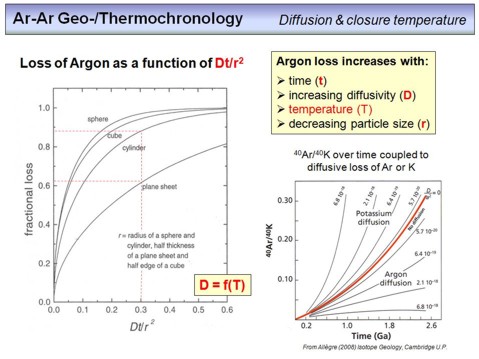 This overhead illustrates the influence of different parameters on the loss of argon from a mineral. We have essentially three parameters that decide whether the argon produced in a K-bearing mineral resides within this mineral or whether it diffuses out and thus gets lost. The first parameter is the diffusivity D, which is strongly dependent on temperature. The higher this value, the stronger will be the Ar-loss. The second parameter is time (t). This means that the argon loss from a mineral is the stronger, the more time is available. This is important if we consider a mineral with an age of, for example, 30 Ma that is reheated during a metamorphic process. The higher the metamorphic temperature, and the longer the duration of metamorphism, the more argon will be lost from our mineral. The third parameter is the size (r) of a mineral (note that r stands for radius, but is used as a measure for any length). The larger a mineral, the longer it takes for argon to pass through it. If we combine all three parameters, then the diffusive loss of argon from a mineral is proportional to Dt/r2. This is the parameter on the x-axis of the diagram on the left. It means that the loss of argon is the larger, the larger D and t, but is inversly proportional to the square of r. In other words, if t and D increases, this can be compensated by an increasing r. The lines in the diagram are loss curves for different geometries as a function of Dt/r2. Note that a fractional loss of 0.6 means that 60% of argon are lost at a given Dt/r2. Assuming a plane sheet geometry, you can see that for Dt/r2=0.3 about 62% of the argon in a grain gets lost by diffusion. For a cylindric geometry, for example an elongated hornblende mineral, at the same value, nearly 90% of argon gets lost. This is because for plane sheets diffusion is only considered in one direction, normal to the boundaries. Regarding this, see this
exercise (loss time).
This overhead illustrates the influence of different parameters on the loss of argon from a mineral. We have essentially three parameters that decide whether the argon produced in a K-bearing mineral resides within this mineral or whether it diffuses out and thus gets lost. The first parameter is the diffusivity D, which is strongly dependent on temperature. The higher this value, the stronger will be the Ar-loss. The second parameter is time (t). This means that the argon loss from a mineral is the stronger, the more time is available. This is important if we consider a mineral with an age of, for example, 30 Ma that is reheated during a metamorphic process. The higher the metamorphic temperature, and the longer the duration of metamorphism, the more argon will be lost from our mineral. The third parameter is the size (r) of a mineral (note that r stands for radius, but is used as a measure for any length). The larger a mineral, the longer it takes for argon to pass through it. If we combine all three parameters, then the diffusive loss of argon from a mineral is proportional to Dt/r2. This is the parameter on the x-axis of the diagram on the left. It means that the loss of argon is the larger, the larger D and t, but is inversly proportional to the square of r. In other words, if t and D increases, this can be compensated by an increasing r. The lines in the diagram are loss curves for different geometries as a function of Dt/r2. Note that a fractional loss of 0.6 means that 60% of argon are lost at a given Dt/r2. Assuming a plane sheet geometry, you can see that for Dt/r2=0.3 about 62% of the argon in a grain gets lost by diffusion. For a cylindric geometry, for example an elongated hornblende mineral, at the same value, nearly 90% of argon gets lost. This is because for plane sheets diffusion is only considered in one direction, normal to the boundaries. Regarding this, see this
exercise (loss time).
The diagram in the lower right illustrates the evolution of the 40Ar/40K ratio in a mineral over time. The red line is the normal evolution, if no diffusion occurs. The lines above the red line are evolution curves for cases where K is lost from the mineral by diffusion, for different values of D. As you can see, this would yield ages that are too old. The lines below the red line are cases where argon diffusive lost occurs. The growth of the ratio is attenuated, and the ages you would get in this case are too young.
Overhead 21
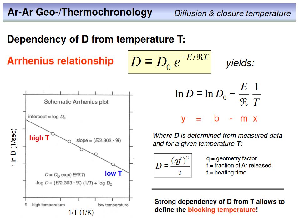 Now to one of the most important things, the relation between temperature and diffusivity. This relation can be described by the Arrhenius relationship, shown here in the yellow box with E = activation energy of the diffusion process (imagine that you need a minimum amount of energy to move an atom from one interstitial position to another interstitial position), R = gas constant, T = temperature, and D0 = frequency factor. This relationship is a function f(x)=e-1/x. This means that for x>0 f(x) increases non-linearly with increasing x. Exactly that is the case for D. With increasing temperature T (i.e. with the exponent becoming smaller), the diffusivity D increases non-linearly. Or, in other words, if a system heats up, diffusion is getting faster. To linearize the Arrhenius relationship, rearrange the equation in a way that lnD = f(1/T). Then, in a plot 1/T versus lnD, as shown on the overhead, the relation between temperature and diffusivity becomes a linear relationship with the y-axis intercept being D0, and the slope being negative with a value of -E/R. Here is an
exercise (Arrhenius) related to this topic.
Now to one of the most important things, the relation between temperature and diffusivity. This relation can be described by the Arrhenius relationship, shown here in the yellow box with E = activation energy of the diffusion process (imagine that you need a minimum amount of energy to move an atom from one interstitial position to another interstitial position), R = gas constant, T = temperature, and D0 = frequency factor. This relationship is a function f(x)=e-1/x. This means that for x>0 f(x) increases non-linearly with increasing x. Exactly that is the case for D. With increasing temperature T (i.e. with the exponent becoming smaller), the diffusivity D increases non-linearly. Or, in other words, if a system heats up, diffusion is getting faster. To linearize the Arrhenius relationship, rearrange the equation in a way that lnD = f(1/T). Then, in a plot 1/T versus lnD, as shown on the overhead, the relation between temperature and diffusivity becomes a linear relationship with the y-axis intercept being D0, and the slope being negative with a value of -E/R. Here is an
exercise (Arrhenius) related to this topic.
Be aware that diffusion parameters in minerals have to be determined experimentally. One has to determine D for several different values of T. This data then can be plottet in terms of ln(D) vs. 1/T, and from the y-axis intercept and the slope one can determine D0 as well as E. Watch the next overhead for an example.
Overhead 22
Here we have an example of how the D value in plagioclase varies with temperature. Shown are two experimental series, one using a larger grain size fraction (490 µm, green points), and one using a smaller grain size fraction (320 µm, blue points). Each point represents an experiment where D has determined at a corresponding T. As you can see, the slopes of both correlations are similar and hence the activation energies for both plagioclase types are similar, but the intercepts and hence the D0 values are different. This is due to different chemical compositions of the plagioclase fractions, and due to different structural features. Note that real crystals are very complicated structures, where phase transitions occur during laboratory heating, and hence assuming simple volume diffusion processes is a strong oversimplification. The deviation from non-linearity in the Arrhenius plots shown here are commonly interpreted as reflecting structural transitions during laboratory sample heating.
Overhead 23
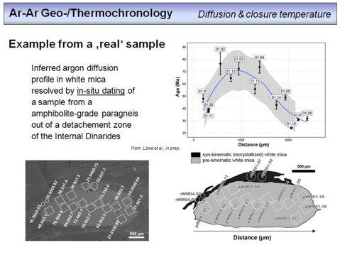 If the Ar isotope composition in a mineral is measured applying methods with a high spatial resolution, such as laser ablation noble gas mass spectrometry (LA-NGMS), age variations can be resolved in an intra-granular scale. This is shown here. The BSE micrograph in the lower left displays a muscovite grain on which 17 spots have been dated using in-situ LA-NGMS, the numbers denote the corresponding Ar-Ar spot ages along with their errors. As you can see, a comparatively large age variation with ages from ~76 Ma to ~16 Ma has been obtained. The interpretation is shown in the lower right. The most largest part of the mica is interpreted as being a pre-kinematic mica, with an age ~75 Ma, the cooling age of the protolith. Younger ages in this part of the grain (bright grey) reflect diffusive loss of radiogenic argon during later stage metamorphism (see the diagram in the upper right where the ages are shown along a profile through the grain). The metamorphic overprint took place at ~16 Ma as is evident from the younger, syn-kinematically grown mica shown in black in the lower right figure.
Overhead 24
This overhead provides frequency factors D0 and activation energies Eα for different biotites, muscovite and hornblende, and the corresponding references. Note that for biotite both parameters are strongly dependent on the Fe/Mg ratio, but also note the huge discrepancy between the values provided by Harrison et al. (1985) and Grove & Harrison (1996), both determined on biotite with 56 mol% annite (the Fe end member of the biotite solid soultion series). This demonstrates the difficulties in determining these parameters in laboratory experiments.
Overhead 25
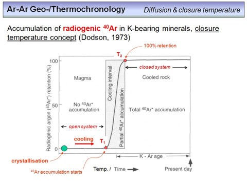 With all the knowledge about diffusion and the temperature dependence of this process, we can do the following thought experiment. Imagine a K-bearing mineral that crystallizes from a magma or that forms during metamorphism by a solid-solid reaction (the green point in the diagram). If the temperature is high (>500-600°C), that means diffusion is fast, any 40Ar that will be produced from the decay of 40K will diffuse relatively fast through the lattice of the mineral to the grain boundary, and there will be lost. The condition required here is that the 40Ar concentration in the pore space is always zero, i.e. any 40Ar production inside the grain will produce a concentration gradient that causes the 40Ar to diffuse out of the grain. If our mineral cools, diffusion will slow down, and at a certain temperature (T1 in the diagram) diffusion will be so slow that 40Ar starts to accumulate inside the grain. Nevertheless, at this point still a significant amount of 40Ar will be lost. If our grain further cools, diffusion is getting slower and slower, and the 40Ar loss gets smaller and smaller. We call this range the partial retention zone, which is the temperature intervall within some of the 40Ar is retained, and the other part is lost. The lower the temperature, the larger the retained amount of 40Ar. At some point, which also corresponds to a certain temperature T2, diffusion will be so slow that it gets insignificant in relation to the 40Ar produced, and from this point we have a closed system. Therefore, the diagram on this overhead displays the retained amount of 40Ar in a certain mineral as a function of temperature. Not that the temperatures T1 and T2 depend on the diffusion parameters of each mineral, and the difference between T1 and T2 is a function of the cooling rate.
Overhead 26
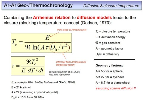 Based on the considerations outlined before, M.H. Dodson (M.H. Dodson, 1973, Closure temperature in cooling geochronological and petrological systems, Contrib. Mineral. and Petrol., 40, 259-274) has developed a concept that attributes a closure temperature to any specific mineral type. The closure temperature Tc describes the temperature at which the effective diffusion rate of Ar in a mineral phase will be that low that the mineral behaves as a closed system. In other words, the closure temperature of a mineral is the temperature, at which the geologic clock starts ticking. The formula(s) to calculate the closure temperature of a specific type of mineral from its diffusion parameters is shown on this and the next overhead. It is very important to know that the closure temperatures for the K-Ar (and thus the Ar-Ar) system in all commonly used minerals are far below magmatic temperatures. Therefore, K-Ar and Ar-Ar ages are usually cooling ages and not crystallisation ages.
Let me provide an example. From a granite, zircon and biotite were separated. The zircons were dated to be 517 Ma by the U-Pb method, whose closure temperature is above 1000°C for zircon. As a granite crystallises from its melt at temperatures between 750-850°C, the zircon age is a crystallisation age because the U-Pb clock starts ticking once the zircon is there. Biotite that crystallises simultaneously or slightly later than zircon from a granitic melt at temperatures in excess of 650°C has a closure temperature of only 350-400°C. This means that upon its existence the biotite will loose all its radiogenic 40Ar due to diffusion until the granite cools below 350-400°C. Within this temperature range the biotite will become a closed system, and therefore the K-Ar or Ar-Ar age of the biotite, let it be 512 Ma, dates the time of closure, not of crystallisation. It is therefore a cooling age. From the time difference of 5 Ma between the zircon U-Pb and the biotite K-Ar (Ar-Ar) age we can infer that it took about 5 Ma for the granite to cool down from its crystallisation temperature to 350-400°C. Note that for volcanic rocks that cool very fast after eruption, K-Ar and Ar-Ar ages can be regarded as crystallisation ages, although they are always cooling ages.
Overhead 27
Note that the closure temperature Tc of a mineral species is a function of the size of the mineral, its geometry (whether a sphere, cylinder or plane sheet, considered by the so called geometry factor), and the cooling rate dT/dt of the rock or mineral. The latter is a bit strange as this parameter is usually not know, but intented to be determined. Nevertheless, its assumption is required to calculate Tc. If you watch the equation on this overhead you will find another strange thing, namely the fact that Tc occurs on both sides of the equation, once in linear and once in a quadratic form. This circumstance requires a numeric (iterative) solution of this equation, which can manually be done by simply assuming an arbitrary value for Tc as a starting value, and then calculating and comparing both sides of the equation. If both sides differ, the value for Tc has to be changed until the difference is sufficiently small. Doing this is the goal of the next
exercise (closure temperatures).
Overhead 28
As you have seen, one can calculate the Tc for a specific mineral type from its diffusion data by an trial end error approach. Clearly, however, an iteration can be done very easily by a computer program. Such a program was written by Mark Brandon and is called 'CLOSURE'. You can download the program for Windows
here.
It solves the Tc equation and has a number of thermodynamic data for different minerals and different chronometers stored already. You just have to choose the chronometer and mineral, the diffusion length in µm (i.e. the radius of a sphere or cylinder), and then the program provides the closure temperatures for a series of cooling rates. To check this out is subject to the next
exercise.
Overheads 29 & 30
These tables provides an overview about approximate closure temperatures as often usedin the literature. As you have seen, the knowledge of diffusion parameters, approximate cooling rates as well as grain size geometry and dimension allows a much better estimate. Note that the K-Ar (and Ar-Ar) systems are 'middle-temperature chronometers' (except for K-feldspar which is a very special mineral with respect to diffusion), whereas the (U-Th)/He and fission track (FT) systems are low-temperature chronometers. Both of the latter will be subject to the second part of this course.
Overhead 31
This nice graphic provides an overview of many different isotope chronometers applied to different minerals, with their inferred closure temperature range. Note that the fission track technology is not an isotope chronometer but rather uses fission induced lattice damage, whereas OSM (optically stimulated luminescence) uses thermally or optically stimulated electron relaxation in quartz, a process where electron transitions from exited to ground state and associated photon emission intensity is a function of (burial) age.
Overhead 32
This overhead gives an example where a cooling path of a piece of rock, for example a biotite-muscovite gneiss, was deduced from applying Rb-Sr, K-Ar and fission-track methods on muscovite, biotite, zircon and apatite that all were recovered from this rock. Note the initaially very fast cooling (~60-80°C/Ma), followed by slower cooling in the low-temperature range (~15-20°/Ma). Such a cooling path might be typical for exhumation processes that balance isostatic disequilibrium without significant tectonic 'disturbance'. Imagine what happens in the case of an overthrust, as schematically shown in the lower part of the left figure, if you sample across the fault? Which part will provide the younger age, the thrusted or the overridden one? Think about the disturbance of the temperature distribution upon overthrusting. Which part cooles faster, which one slower? From thinking about such questions you will become an idea on how thermochronology can be used to reconstruct tectonic processes.
Overhead 33
This overhead shows the cooling path of a syenite intrusion as deduced from different minerals recovered from a single specimen, and by applying different thermochronometric methods. As you have seen before, the trick is to combine different minerals and different chronometers. This is a huge piece of work, but provides quantitative data on geological processes. In this example, from the cooling rate of the pluton one can deduce the intrusion depth from thermal modelling, given that superimposed tectonic processes are slow or negligible.
Overhead 34
Here an example where the thermal history of a detachment fault was reconstructed by applying different middle- to low-temperature chronometers. The lower left diagram displays the result of the application of common 'bulk-closure' chronometers, which leave a gap in the thermal history between ~50 to ~15 Ma. Applying more sophisticated hence controversially discussed continuous temperature-time (T-t) chronometers such as K-felspar multi-diffusion domain thermal modelling (MDD) and fission track length distribution thermal modelling fills this gap and reveals unsteady cooling in this time interval, with slow cooling from ~60-45 Ma and ~33-15 Ma, but rapid cooling from ~45-33 Ma and from ~15 Ma on. The fast cooling events are interpreted to reflect 3-4 km of denudation during Eo-oligocene times, and ~6 km of footwall exhumation from ~15 Ma on, the latter in response to the opening of the Gulf of California.
Overhead 35
 Until now we have learned about the basics of the K-Ar method, and about a number of applications of thermochronology in earth sciences. You might have noticed that the examples from the literature rather used the results from the Ar-Ar method instead of the K-Ar method, for which the same principles regarding diffusion and closure temperature are valid. But what is the difference between these two methods? The answer is fairly simple, both methods differ only in the way by which the K-content of a sample is determined. That's basically all, but as you will see, this tiny modification has a hughe impact!
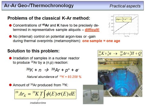
The overhead lists the two major disadvantages of the K-Ar method. The first is the fact that 40Ar and K concentrations have to be determined on a rock or mineral, which is very difficult to achieve with high precision and accuaracy. Both elements have very different chemical behaviour, K is a metal and Ar is a noble gas, and therefore their concentrations in representative sample splits have to be determined independently from each other. This can be by solution-based atomic absorption spectroscopy (AAS) or mass-spectrometry for K, and by isotope-dilution noble-gas mass spectrometry for Ar. In particular the latter is associated with very complicated and difficult laboratory routines. Easily speaking, the need to apply different methods and to determine absolute concentrations of two different elements results in relatively large uncertainties, and thus in comparatively unprecise ages.
The second disadvantage is that the K-Ar method does not provide an internal control whether a sample has lost some of its argon in the geologic past, or has gained any argon during, for example, metamorphic processes. Easily speaking, applying the K-Ar technique, we get only 'one age' from 'one sample'. As you will see later, the way in which an Ar-Ar age is determined provides a strong control on its overall reliability. In other words, by adopting the technical treatment, it is possible to gain much more data out of a sample and hence more information on its (geologic) history.
To overcome these problems, the Ar-Ar method has been developed. The difference to the K-Ar technique is that samples were irradiated with neutrons in a nuclear reactor, usually a research reactor. The Argonlab Freiberg, for example, uses the
LVR-15 Research Reactor
of the Research Centre in Rez, Czech Republic, for sample irradiations. This reactor uses enriched (19.8%) 235U-fuel and provides a maximal thermal power of 10 MW at a maximal thermal neutron flux of 1014 neutrons per second and per cm2 (i.e. 1014 n/cm2s, this means that 1014 neutrons cross an area of 1 cm2 every second). Note that 'thermal neutrons' refers to a specific energy range (spectrum) of neutrons (details see
here).
Irradiating a K-bearing rock or mineral with neutrons causes nuclear reactions of the target isotopes, and the required reaction in our case is the transformation of some of the 39K in a sample to 39Ar. This transformation is by a so called (n,p) nuclear reaction where a neutron enters the core of a 39K isotope. Due to neutron excess such a core is unstable and therefore in turn emits a proton to become stable again. The net effect is a constant mass but an ordering number reduced by one such that the new element is argon, or, to be more precise, the 39Ar isotope. Note, that 39Ar does not occur in nature in noteworthy amounts (there is some cosmogenic 39Ar in the atmosphere, but due to the short half life of 39Ar of 269 years this amount is extremely low).
The amount of 39Ar produced in a K-bearing rock or mineral is proportional to the irradiation time (T), the neutron flux (φ) and the K-concentration. In other words, irradiating samples to be dated with neutrons prevents us from the need to determine the K-concentration of this sample. Instead, we simply need to measure its argon isotope composition and from this can calculate an Ar-Ar age. In this context note that it is orders of magnitude more simple to measure the isotope abundances of an element than its absolute concentration!
The integral equation on the bottom of this overhead allows to calculate the amount of 39Ar produced from 39K by irradiaton (we call it 39ArK). T is the irradiation duration, φ is the neutron flux and σ is the
reaction cross section
of the 39K(n,p)39Ar reaction, where both of the latter depend on the energy distribution of the neutrons. This is the reason why we need to integrate over the whole neutron energy spectrum to become 39ArK.
Overhead 36
This is an image of the LVR-15 reactor in Rez, a view from the top of the reactor vessel into the reactor core with the U-fuel elements. The blue light is
Cherenkov radiation
(Tscherenkow Strahlung) whose emission results from the slow down of the velocity of electrons that enter a dielectric medium, in this case water, with a velocity higher than the velocity of light in this medium. It is characteristic for liquid cooled nuclear reactors. You can also see the metal tubes that direct down into the reactor core. These tubes were used to bring down sample material into the core for neutron irradiation.
The image on the lower left is an aluminium plate with a diameter of 33 mm with holes in it. The samples for Ar-Ar dating were placed in such plates, before several of them were stacked together (image on the lower right) to be irradiated. For irradiation, a sample batch that contains as much as 70-100 samples is placed close to the core of the reactor.
Overhead 37
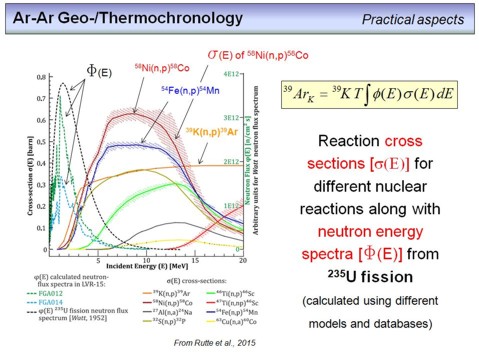 Back to the theory of the irradiation procedure. This somewhat busy diagram shows two things. First different neutron energy spectra (denoted ΦE), one from the literature from Watt (1952), this is the black dashed line. And then two other energy spectra that have been determined and modelled for the LVR-15 reactor (the blue and green dashed lines, labelled FGA012 and FGA014). The neutron flux is given at the right hand y-axis and you can see that the maximum of the theoreticall calculated neutron flux that results from the fission of 235U is at about 2 MeV (the black dashed line from Watts, 1952). This theoretical maximum coincides roughly with the measured and modelled energy spectrum of the LVR-15 reactor (green and blue dashed lines).
The second set of curves shows reaction cross sections (the unit is barn, 1 barn = 10-24 cm2) of a number of nuclear reactions. The higher the reaction cross section, the higher the likelihood that the corresponding nuclear reaction takes place. As you can see, the reaction cross section is also a function of the neutron energy, and 'our' reaction, the 39K(n,p)39Ar-reaction (orange line), only takes place at a significant rate if the energy of the neutrons exceeds ~1.3 MeV. This means that we need 'fast neutrons' to perform the transformation of some of the 39K to 39Ar.
The other reaction cross section curves are only for comparison and are given for metals that are frequently used as neutron flux monitors in nuclear physics.
Overhead 38
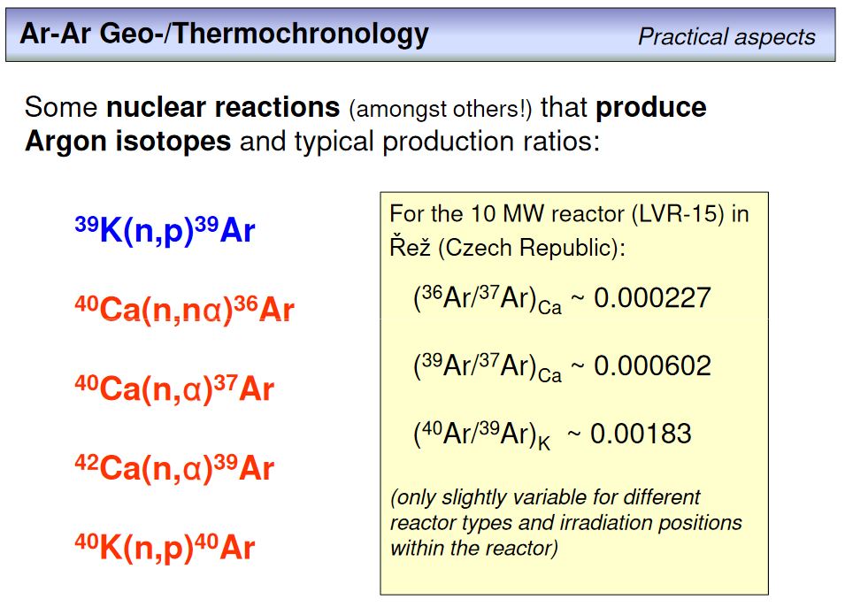 As said, there is not only 39K that undergoes a nuclear reaction upon neutron irradiation, basically all chemical elements will be affected. This is not what we want, but there is no possibility to prevent this negative side effect (indeed Cd-shielding reduces such competing nuclear reactions, but a complete suppression is not possible).
This overhead shows some nuclear reaction that are relevant in Ar-Ar dating. The first one, in blue, is the reaction that we want to have. However, the reactions in red are also relevant, however, since they produce different Ar isotopes. You remember from overhead #6 that only three Ar isotopes exist, namely 36Ar, 38Ar and 40Ar. Here you can see, that 36Ar and 40Ar are produced from Ca and K isotopes. This means that if a sample contains radiogenic 40Ar* plus atmospheric argon with all three isotopes and their respective abundances, the irradiation process will further add additional 36Ar and 40Ar from 40Ca and 40K. Moreover, 37Ar and additional 39Ar will also become part of our sample because of nuclear reactions of 40Ca and 42Ca. In the end you can see that the isotope composition of argon in an irradiated sample is a complex mixture of initial argon, atmospheric argon, nucleogenic argon and radiogenic argon. To calculate an age from an irradiated sample requires to decipher this mixture, but we will come back to this later in overhead #50.
Note, however, the following. If pure Ca is irradiated, or a very pure CaF2 sample, then only Ca-based argon isotopes will be produced, i.e. 36Ar, 37Ar and 39Ar. The important thing is that the production rates are very different, but constant relative to each other. Therefore, we can define Ar-isotope production ratios from Ca, as is shown on the right hand side of the overhead. The same can be done with any other elements, but K and Ca are the most important ones, as many minerals contain not only K but also lots of Ca (hornblende, plagioclase, whole-rocks). Keep this in mind, we'll need it later.
Overhead 39
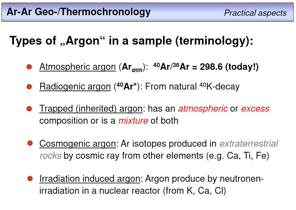 Before we'll have a look on more practical aspects of Ar-Ar dating, this overhead summarizes the 'types' of argon that need to be distinguished to understand the interpretation of Ar-Ar data. Note that each 'argon component' has its own isotope composition, a circumstance that is clearly invisible! Take the isotope composition of atmospheric argon, that is of the argon that is part of the air we breath. The isotope abundances of atmospheric argon is known (see overhead #6), and from these isotope abundances we get the following isotope ratios: 40Ar/36Ar ~ 296.1, 40Ar/38Ar ~ 1575.9, and 38Ar/36Ar ~ 0.1879. Note that these are only rough numbers where it is assumed that all Ar-isotopes have the same weight. A precise calculation would require to recalculate the weight% amounts to moles, an exercise that you have done already.
Beside atmospheric argon there is radiogenic argon, trapped argon, cosmogenic argon and irradiation induced argon. Trapped argon is any argon that is incorporated in a rock or mineral other than radiogenic argon and thus might be initial argon or argon that was incorporated later, e.g. during metamorphism or simply during lab handling, and mostly inherited argon is a mixture of both. If the initial (or in the end trapped) argon of a rock or mineral has a 40Ar/36Ar ratio >298.6 (this is the atmospheric value), then it is called excess argon because it contains a radiogenic component (excess) that was not produced by K-decay within this rock or mineral. In extraterrestrial samples there are argon isotopes produced by cosmic rays from other elements, similar to what happens during neutron irradiation that produces irradiation related argon.
Overhead 40
With all the theory in mind, we now will have a look on more practical aspects of Ar-Ar dating. In some way, the argon needs to be released from a rock or mineral, then it needs to be cleaned before its isotope abundance can be determined by a noble-gas mass-spectrometer. All process take place under a very high vacuum better than 1 x 10⁻⁸ mbar. Gas release from a sample is usually achieved thermally by a furnace or a thermal laser (that is a laser with a wavelength in the infrared range), by 'cold ablation' using an UV-laser, or meachnically by using a crusher (if, for example, fluid inclusions or gas bubbles need to be analysed). Note that not only noble gases such as Ar are released from a rock or mineral, but also other gases such as H2O, CO2, CO, HCl, HF, hydrocarbons, etc., such that gas cleaning is necessary (otherwise we will not have a stable signal in the mass spectrometer due to competing ionization effects). Gas cleaning can be achieved using cold traps, e.g. with liquid nitrogen, or with so called 'getter pumps' (see below). After cleaning, where all but the noble gases have been eliminated from the gas-mixture, the Ar is expanded into a noble-gas mass-spectrometer (NGMS) where its isotope abundances are determined.
Overhead 41
This photograph shows a New Wave CO2-laser system that is used for thermal gas release. The laser is a floating system positioned above a sample chamber, in which the rocks or minerals are loaded on copper discs in holes. Moving the laser by a motorized stage allows automated positioning and heating of individual samples. The wavelength is in the far infrared (10.6 µm) to perform efficient heating of all type of material.
Overhead 42
The lower left image shows a close up view of the laser sample chamber. It consists of stainless steel and is equipped with an infrared transparent ZnS-window that is flanged onto the sample chamber. The lower right figure shows the sample chamber with the window demounted. You can see the copper sample holder that, in this case, takes up thirty samples, rock or mineral splits, ~3-4 mg of each per hole. The whole sample holder is covered by a 1 mm ZnS-window to protect the main window from condensating silicate vapour. The image on the upper right shows the loading procedure of the sample holder. A special device has been manufactured to enable sample loading without cross-contamination.
Overhead 43
This overhead shows the Freiberg furnace system (HTC = high temperature cell) that was developed and build in cooperation with
Createc Fischer.
The system is unique and provides significant advantages such as a small volume and low-blank levels due to the ability to remove measured samples out of the vacuum-system. Details along with more general inforamtion about ALF can be found
here. Very briefly, rock or mineral splits up to 1000 mg were loaded into Mo-crucibles and stored in a vacuum-sample chamber. From this chamber, each sample crucible can be transferred by a mechanical system under high vacuum down into the HTC (furnace) to perform step-wise heating. After degassing, the sample residue can be retranserred back into the sample chamber before the next sample is measured.
Overhead 44
Gas cleaning is typically achieved using two 'getter pumps'. These pumps adsorb and absorb all kinds of active gases including H2. They consist of a zirconium-based metal alloy coated as a metal powder on carrier plates of steel to achieve a large surface. Inside the getter devices, a heating element is used to regenerate the getter surface (at ~700°C), and in normal operation at ~400°C to crack larger molecules to smaller ones to get adsorbed or absorbed by the alloy.
Overhead 45
This overhead displays the pumping speed of an St101 getter alloy from SAES (Milano, Italy) for different gases at different temperatures. The x-axis provides the sorbed (sum of adsorbed and absorbed gases) quantity of gas in [Torr x Liters]. Note that 'Torr' is an old unit for pressure where 1 Torr = 133 Pa = 1.33 mbar. As you can see, the pumping speed is highest for hyrogen, and slowest for CO at room temperature. This is important to consider to provide enough time for gas cleaning. In our lab we use gas cleaning times of 5 minutes. Note that any active gases such as H2O, CO, and CO2 in the ion source of a mass-spectrometer will cause chemical reactions at the hot filament to form hydrocarbons that may isobarically interfere with Ar masses (e.g. C3H3+ on mass 39).
Overhead 46
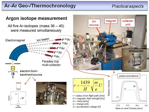 This overhead provides a very brief overview about noble-gas mass-spectrometry. A NG-MS consists of an ion source, a sector field magnet and a detection system. The gas once expanded into the mass spectrometer gets ionized by an electron bombardement source, where the electrons were emitted by a hot filament. Acceleration and focussing of the ion beam is achieved by high-voltage electrostatic fields (the ion optics of the source). The ion beam is transmitted through a magnetic field orthogonal to the magnetic flux lines, which leads to a mass-dependent dispersion of the ions according to the Lorentz force acting on them. A detection device positioned in the focal plane of this ion-optical system allows either a sequential detection of the intensity of each ion-beam by 'switching' the magnet field strength (peak hopping), or a simultaneous detection of all five argon masses (36Ar to 40Ar) by using five detector units (a so called static measurement as shown on the overhead). The detection devices are typically either 'Faraday cups' or if higher sensitivities are required secondary-electron multiplier (SEM) based devices. The intensity of each ion-beam, i.e. the voltage or current provided by a Fraday cup is directly proportional to the number of ions entering the cup per time.
The formula given on the overhead allows to calculate the radius of the flight path of an ion as a function of the strength of the magnetic field, the mass of the ion, its charge and the acceleration voltage. Note that the flight path radius of an 40Ar++ ion is half of that of an 40Ar+ ion. Any multiply charged Ar ions will therefore not be detected.
The figure on the lower right shows five argon signals as recieved by a simultaneous measurement of all five argon masses on five Faraday cups. The peaks are flat-top peaks, an important feature to perform high-precision isotope ratio measurements. The numbers denote the masses of the corresponding Ar isotope. Let's close this more technical part with an
exercise.
Overhead 47
With the knowledge about the measurement principles of argon extracted from irradiated rocks or minerals, we need to think about how to calculate an age from the measured isotope abundances. Adopting the overall radioisotope age equation (1), valid for all decay systems, with daughter being 40Ar* and parent being 40K, we get equations (3) and (4) where f consideres the amount of 40K that decays to 40Ar* (remember the branching ratio; see overhead #4).
Overhead 48
With the known abundances of K-isotopes, any present-day 40K amount (moles!) can be recalculated to 39K, this is equation (5). As derived in overhead #35, the amount of 39Ar from 39K (abbreviated as 39ArK) produced during irradiation can be expressed as given in equation (6). Taking the time of irradiation and the integral term together and defining it being J', equations (5) and (6) combine to equation (7). Inserting equation (7) into equation (4) yields equation (8).
Overhead 49
Taking all constants in equation (8) together and making them the new constant J, we get the age equation of the Ar-Ar technique. Using this equation, an age can be calculated from the measured argon isotope composition of an irradiated rock or mineral, if the 40Ar*/39ArK ratio is obtained. Note that the constant J has also to be known, it is typically called J-value or irradiation parameter. As this parameter can not be calculated precisely, it needs to be determined from minerals with a known age that were irradiated along with the samples of unknown age. Such mineral standards were called fluence monitors as they quantify the neutron flux (and fluence) of any specific irradiation. But note that any other constants used are also included in the J-value.
Overhead 50
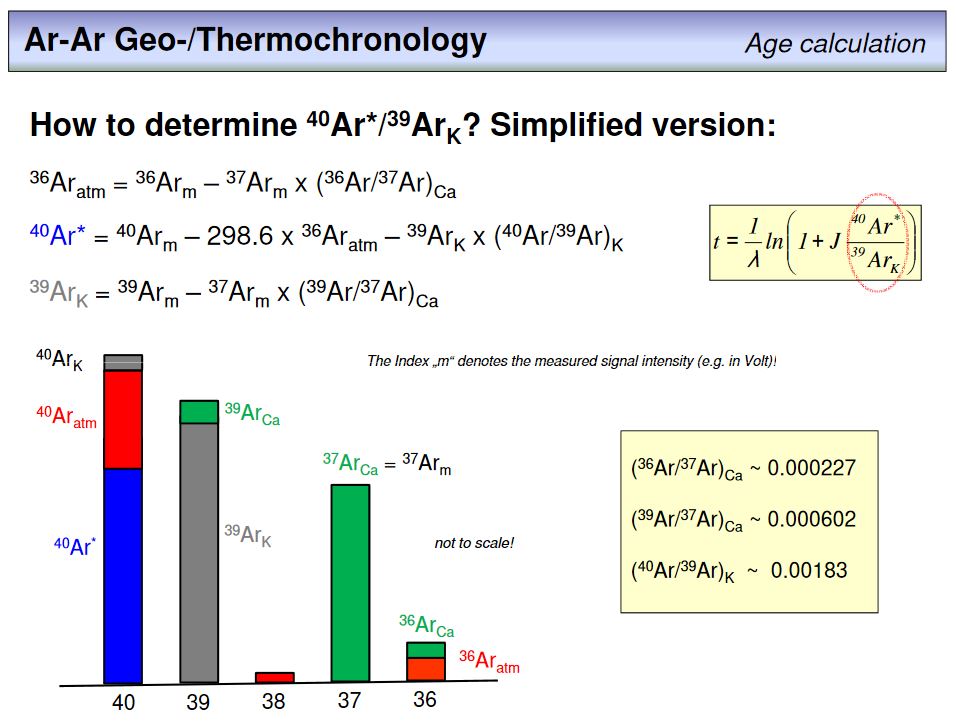 The question now is how can we get 40Ar*/39ArK from measured argon isotope intensities? To resolve this, watch the figure. The bars represent the measured signal intensities in the mass range 36 to 40. Most of the signals comprise different components, and the task is to sort them out. This can be done by known ratios. Let us take the measured signal on mass 36. This is 36Ar from an atmospheric component, and 36Ar produced from Ca during irradiation (see overhead #38). In the case of 37Ar, the measured signal intensity is solely from 37Ar produced from Ca. As we know the production ratio of 36Ar to 37Ar from pure Ca, which is ~0.000227 (overhead #38), we can calculate the Ca-related contribution to the measured 36Ar signal (the green part) and subtract it from the total signal. The difference is the atmospheric component (the red part), which in turn can be used to correct for the atmospheric contribution to the measured signal (from the knwon atmospheric 40Ar/36Ar = 298.6 ± 0.3). In the same way the 39 signal can be corrected for 39Ar from Ca, and then using this value enables to correct the remaining 40Ar signal for irradiation induced 40Ar from K. There are some more corretions required that include also 38Ar, but the principle is overall the same. Having done all these corrections we end up with the required 40Ar*/39ArK value, from which we can calculate the age of a sample.
Overhead 51
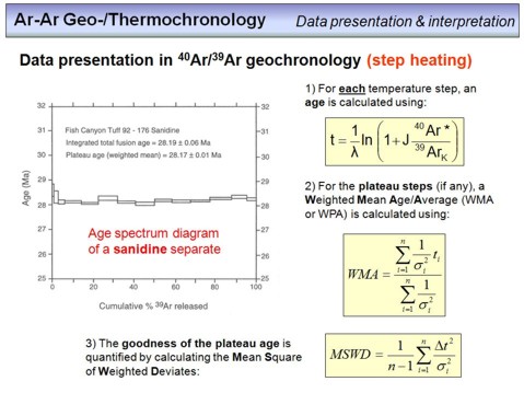 Heating of a rock or mineral sample to extract argon is usually not done in a single step, but in several steps where the temperature is increased from step to step. For each step, the released argon is cleaned and measured. This procedure is time consuming (~20-30 min per step), but allows to control for internal data consistency as from each step an age can be calculated. This means that a single sample does not provide a single age, but a number of ages from which an overall best age estimate can be derived. One way to display Ar-Ar step-heating data is in the form of an age spectrum. This is shown on the overhead. Each rectangle in the diagram corresponds to a single step, for which an age was calculated. The height of each rectange represents the uncertainty, or error, of the calculated age, and the width represents the amount of 39ArK in percent that is included in this step. The sum of all measured 39ArK intensities from a sample were set to 100%. Usually, the error or uncertainty of a step inversely correlates with 39ArK, as higher signal intensities result in lower signal uncertainties and thus in lower age uncertainties.
In cases where the majority of steps provide an identical age within error (a so called plateau), the age of a sample is usually given as weighted mean average (WMA). To calculate a WMA, the age of each step included in the plateau is weighted by the inverse of its variance. This is the second formula on this overhead. Accordingly, age values with large uncertainties contribute less to the final age than those with little uncetratinties.
An important number that 'measures' the analytical uncertainty relative to the 'geological disturbance' of a sample is the mean square of weighted deviates (MSWD). To understand this number we need to consider the following. Many samples undergo multiple geological events after formation. These can be metamorphic overprints, hydrothermal alteration, submarine alteration and/or weathering. Each event may cause Ar loss or Ar gain (or K loss or gain) to the minerals of a sample, and we call all this simply 'disturbance' as these processes disturb the evolutiuon of our chronometer as a closed system as required from theory. By contrast, our analytical procedures in the lab underlie uncertainties, and any gained value will be associated to an error. The question is the significance of the sum of the analytical errors in relation to the sum of the disturbances. This can be expressed by the MSWD. In cases where the MSWD is ~1, the magnitude of the analytical uncertainty equals approximately the magnitude of the 'geological disturbance'. Generally, this is an ideal case, where an improvement of the analytical capacities would not result in a significant improvement of the result (as this is limited by the geological disturbances). In cases where MSWD > 1 (often >> 1), we have overdispersion, i.e. the geological disturbance exceeds the magnitude of the analytical accuracy. In this case the accuracy of an age (if there is an age at all!) is not limited by the analytical capabilities but by the geological disturbance. In cases where the MSWD is < 1 (or << 1), the limiting factor is the analytical uncertainty and any improvement of the analytical capacities would result in a more precise age.
How is the MSWD determined? Watch the third formula, and let us use the example of an age spectrum diagram. From a number of n steps one can calculate a WMA age. Then the square of the difference between the age of each step and the WMA is calculated (Δt2) and divided by the variance of this step (σ2). The sum of these 'deviates' multiplied by 1/(n-1) is the MSWD value. Watch the following
exercise.
Overhead 52
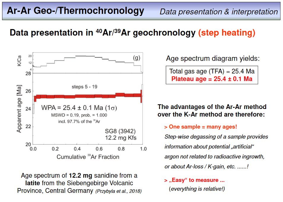 As you have realized in the meantime, Ar-Ar dating is typically not done by total fusion degassing of a rock or mineral split, but by step-wise heating and analysing each released gas fraction. Clearly, the temperature is slightly increased from step to step, and in case of laser heating, this is done by a step wise increase of the laser power. The result of such a step heating experiment is a number of ages out of a single sample, as you have seen already in the last overhead. This overhead provides an example from our lab. The ages of the steps contiguously overlap within error. This is important as it means that we have an internally consistent set of ages from our sample, in this case 12.2 mg of a sanidine separate. This 'consistency' makes the WMA value very likely to be an accurate age within the calculated external reproducibility, and is expressed by a MSWD of 0.19 which further indicats that the analytical precision limits the precision of the obtained age. If one calculates a total fusion age from all steps, this value will be nearly identical to the WMA. Note that the WMA is called WPA here. This means weighted plateau average and is used here instead of WMA as only the red steps (the 'plateau steps') have been included in the WMA age calculation. In this example, the red steps correspond to 97.7% of the total amount of 39ArK released.
To summarize, we can extract several indicators from a step heating experiment that allow to justify the quality of an Ar-Ar age: (1) the error of the age (which is either an internal or external error and calculates from error propagation considering each step during age calculation), (2) the MSWD that quantifies the degree of geological disturbance of an age, and (3) the amount of 39ArK that is included in a WMA or WPA calculation. In general, the error should be as small as possible, the MSWD should be ~1 (or less than 1), and the amount of 39ArK included in WMA calculation should be as large as possible. With using these criteria, the age obtained in this example seems to be a robust and reliable age.
There is something else to be seen here, this is the plot on top of the age spectrum, the K/Ca-plot. What do you think does this plot show? Please provide your answer in the following
exercise.
Overhead 53
This overhead shows the age spectrum of a hornblende separate of which 24 temperature steps have been measured (note that such an experiment requires 12-14 hours of machine time). It looks ugly (...), and clearly no plateau is visible, and therefore no plateau age (WMA) can be calculated. In other words and although a lot of effort was put into this experiment, from hornblende picking to washing, irradiation and finally measurement, no age is obtained and all the effort was in vain. Annoying but true. Note that dating of this hornblende split by using the K-Ar technique would have provided an age of about 140 Ma, likely even with a good analytical precision, but this number is useless as this sample is fully disturbed. This disturbance is invisible by the K-Ar technique, but obvious from the Ar-Ar step heating data and the MSWD of 2377 (!) calculated from it. Note that an Ar-Ar total gas age, or total fusion age (TFA), calculated from the sum of all measured temperature steps always is equal to the K-Ar age of a sample (at least theoretically).
Overhead 54
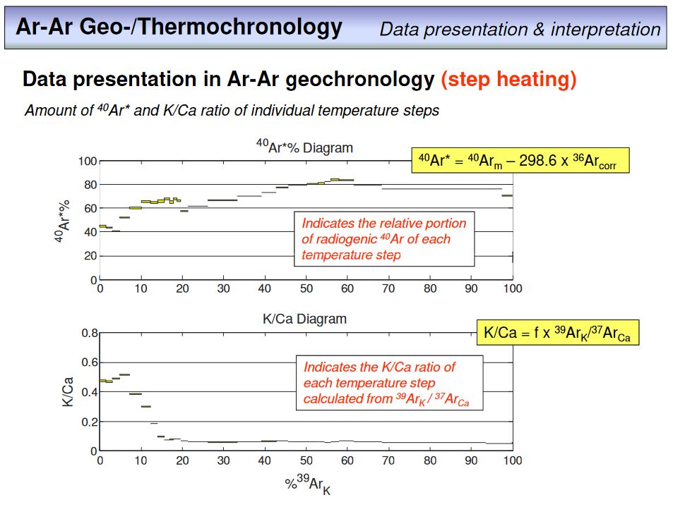 This overhead shows additional data calculated from the measurement results of the hornblende separate whose age spectrum is shown on the previous overhead. As mentioned already, not only age information is obtained for each temperature step, but also a K/Ca ratio of the part or domain of a sample or mineral from which this gas fraction comes from. Even more, based on the Ca-corrected amount of 36Ar measured in each step, we can calculate the percentage of 40Ar* that corresponds to this step (see overhead #50). This is important as the higher the amount of 40Ar* in a step, the lower was the underlying atmospheric correction applied to this step (see overhead #50). In this context it is also important to know that the atmospheric correction imprints considerable uncertainty to the final result as the measured signal intensity of 36Ar in a step is usually very low, and thus comparatively unprecise. This 'unprecision', however, is multiplied by 298.6 in the course of doing the atmospheric correction on the measured 40Ar signal, and thus is disproportionately high propagated into the final age uncertainty. Simply speaking, the higher the amount of 40Ar* in a step, the better. The same, by the way, is valid for the K/Ca ratio of a step. The higher this value the better, as for high K/Ca the Ca-related interference corrections of the corresponding step have been low. And any correction imprints an additional uncertainty on the final result.
What might the K/Ca plot of the hornblende sample in this example tell us? What do we observe? We observe elevated K/Ca ratios, starting at ~0.5 for the first 4 steps (low temperature steps), which then decrease over steps 5 to 8, and stabilize at a value of ~0.08 from step 9 on (middle to high temperature steps). How can we interpret this observation? A plausibe explanation would be that the hornblende dated in this example was overgrown by another amphibole phase, with a higher K/Ca ratio. Assuming degassing controlled diffusion, clearly a fraction of minerals (with a more or less identical size) will degas successively from its outer rim to its core during a step heating experiment. Hence, the low temperature steps represent the outer parts of a grain, and the middle to high temperature steps the more inner parts of a grain. Therefore, the minerals analysed here had a rim with a higher K/Ca ratio than the inner parts. This rim might represent a retrograde metamorphic overprint. What we further can see is that the inner parts of the hornblende have a very homogeneous K/Ca ratio, from which one would expect a reliable age information, i.e. a well defined plateau. As you can see on the previous overhead, however, this is not the case and the most likely interpretation is that this sample was multiply overprinted during the alpine orogenesis, which lead to partial argon loss during reheating. This partial argon loss further disturbed the sample that likely suffered already by a preexisting excess argon component. To summarize, the combination of partial argon loss processes and the presence of excess and atmospheric argon components made it impossible to derive an age for this hornblende.
Overhead 55
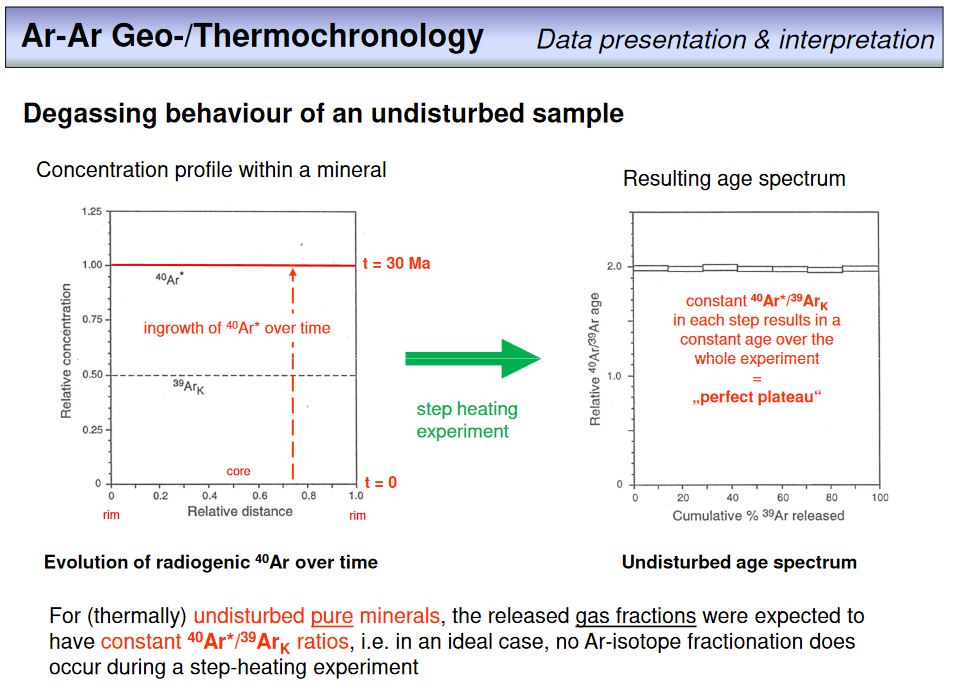 Likely the explanations provided with the last overhead are not easy to understand. Let's therefore in the following think about what happens to a K-bearing mineral over time, and what will happen if thermal events affect their evolution.
Imagine a mineral in which the potassium is homogeneously distributed at the time of its formation. We will call this moment the starting time (t=0). The K-concentration profile across such a mineral will be a horizontal line in a diagram as shown on the left side of this overhead. As the mineral just formed it will be free of any 40Ar*, and thus at t=0 the concentration of 40Ar* is zero. If time goes, 40Ar* will form from the decay of 40K, and this 40Ar* will be homogeneously distributed over the grain as K is also homogeneously distributed. A concentration profile of 40Ar* in our grain will therefore be also a horizontal line in the diagram on the left. This 'horizontal line' will move upwards with time, as 40Ar* becomes more and more. But, it will always be homogeneously distributed over the grain. After a certain time, in our example after 30 Ma, a geologist collects the sample and isolates the mineral, to do Ar-Ar dating. After irradiation, the sample will not only contain 40Ar*, but also 39ArK with a distinct concentration that, however, is also homogeneously distributed over the grain. This is the dashed line in the left figure. If a step heating experiment on this grain is performed, it will degass successively from the outer to the inner parts, i.e. from the rim to the core, but if the system developed completely undisturbed, the 40Ar*/39ArK-ratio in each step, und thus the age of each step, will be the same. The experiment will therefore provide a 'perfect plateau' in an age spectrum diagram, as is shown on the right of this overhead. In this age spectrum, the first steps, i.e. the steps on the left, represent the low temperature steps, and thus the outer parts of the mineral, whereas the last steps, i.e. the steps on the right, represent the inner parts and the core of the mineral (see
this figure).
Overhead 56
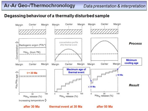 Let's extent our virtual experiment. On the very left you can see what the age spectrum of a mineral would look like if it develops for 30 Ma without disturbance before its getting dated. This is what was described on the previous overhead. But now imagine, the mineral is not sampled after 30 Ma, but underwents low- to medium grade metamorphism that brings the mineral to or above its closure temperature. In this case the mineral will loose 40Ar* (and other argon isotopes if present!) by diffusion, and the diffusion speed and thus the amount of loss is controlled by temperature and time as you know! Clearly, the argon that is in the outermost parts of the mineral will reach the surface first, so the loss of argon will start at the rim and continue to the center of a mineral. Lets assume that the thermal event will not degas the grain completely, but only partly. The concentration profile of 40Ar* will then be, for example, a bell shaped curve as is shown as a dotted line in the middle part of the middle figure. Clearly, dependent on the duration and temperature of the thermal event, the argon loss profile, i.e. the dotted line, will look different. What shapes it might have is to answer in the next
exercise.
Let's extent our virtual experiment. On the very left you can see what the age spectrum of a mineral would look like if it develops for 30 Ma without disturbance before its getting dated. This is what was described on the previous overhead. But now imagine, the mineral is not sampled after 30 Ma, but underwents low- to medium grade metamorphism that brings the mineral to or above its closure temperature. In this case the mineral will loose 40Ar* (and other argon isotopes if present!) by diffusion, and the diffusion speed and thus the amount of loss is controlled by temperature and time as you know! Clearly, the argon that is in the outermost parts of the mineral will reach the surface first, so the loss of argon will start at the rim and continue to the center of a mineral. Lets assume that the thermal event will not degas the grain completely, but only partly. The concentration profile of 40Ar* will then be, for example, a bell shaped curve as is shown as a dotted line in the middle part of the middle figure. Clearly, dependent on the duration and temperature of the thermal event, the argon loss profile, i.e. the dotted line, will look different. What shapes it might have is to answer in the next
exercise.
What an age spectrum will we get if we date our sample directly after the thermal event, i.e. after metamorphism? As K will not be affected by the thermal event, the distribution of 39ArK in the mineral after irradiation will be homogeneous and thus will be a horizontal line in a concentration profile diagram (middle figure). A step heating experiment will therefore provide successively increasing 40Ar*/39ArK-ratios, and thus successively increasing ages in an age spectrum diagram, as degassing proceeds from the outer to the inner parts of a mineral, and as 40Ar* becomes successively more towards the core of the grain. In cases where the thermal loss was limited, the last steps in an age spectrum diagram might form a plateau and this might provide the original formation or cooling age of the mineral.
Let us continue our virtual experiment. What happens if the mineral is not dated directly after metamorphism, but remains for another 20 Ma markedly below its closure temperature? Simply, it will start again to accumulate 40Ar* from 40K decay. The newly produced 40Ar* will again be homogeneously distributed over the grain, and this means that the original loss profile that resulted from the thermal overprint at 30 Ma (or, in other words, 20 Ma ago) will move upwards over time, without changing its geometry. This is shown on the right. If, after another 20 Ma, or after a total time of 50 Ma, the mineral is irradiated and dated, the age spectrum will look as shown in the lower right. In a very ideal case, the low temperature steps in such an age spectrum will provide the upper limit, or maximum age of the thermal event (i.e. the thermal event in our example was 20 Ma ago or less), and the high temperature steps will provide the lower limit, or minimum original age (formation or cooling age) of our mineral. Imagine what would happen if a mineral with an age of 50 Ma would loose 50% of its radiogenic argon in the outer parts at 5 Ma? What an age would be provided by the low temperature steps? 5 Ma? No, ~30 Ma! It would only provide 5 Ma if the outer parts of the mineral were completely resettet during the thermal event!
Overhead 57
With the descriptions before there should be hardly any problem interpreting this step heating diagram that provides a more or less perfect plateau. The sample dated here is a biotite (GA1550) out of a monzonite from the Mt. Dromedary Complex in New South Wales, SE Australia. The well defined plateau indicates that the biotite developed mostly as a closed system after initial cooling.
Overhead 58
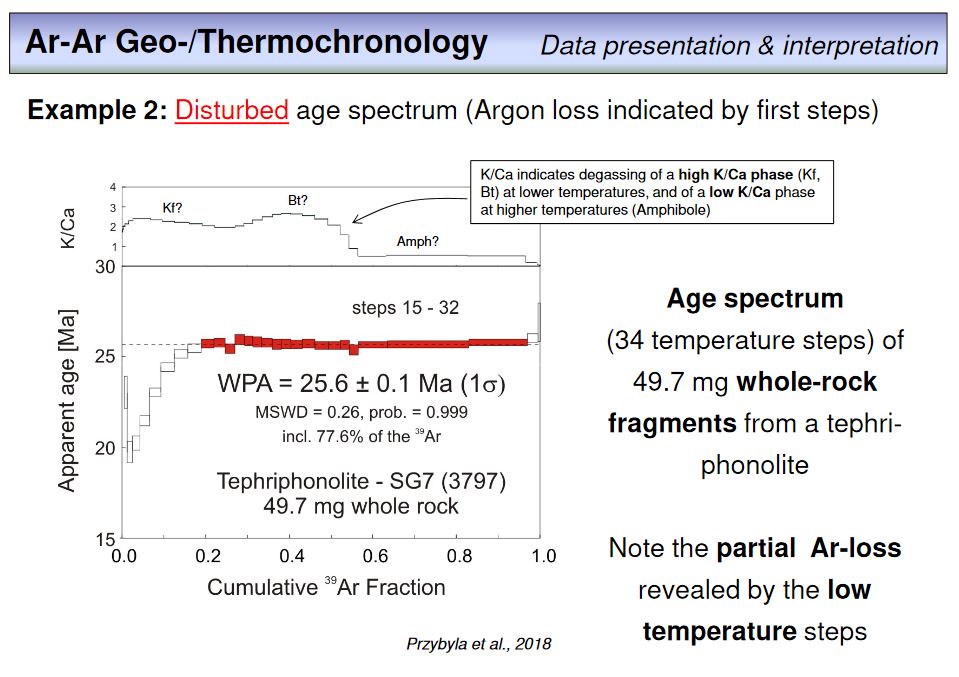 This example shows an age spectrum of ~50 mg of whole-rock fragements (250-500 µm in size) prepared from a tephriphonolite from the Siebengebirge Volcanic Province in Central Germany. The low temperature steps display successively increasing ages, whereas the middle and high temperature steps form a plateau that provides a WPA of 25.6 ± 0.1 Ma from 77.6% of the released 39ArK. The increasing ages can be interpreted as partial argon loss, but the plateau age is likely to present a robust cooling age for this sample. As it is a volcanic rock, the cooling age can be taken equal to the eruption age in this case.
What else can we take out of the data? Watch the K/Ca spectrum in the upper part of the figure and note that not a mineral but a rock was dated here, i.e. a multi-phase system! So, we have a mixture of different minerals with different closure temperatures, but as cooling was fast, their ages might not differ in a resolvable way. In the K/Ca plot you can see that the low to middle temperature steps affected a phase, or phases, with a high K/Ca ratio of ~2-3. This is too low for pure K-feldspar and pure biotite (both have >10), but too high for most amphiboles. So it likely indicates that a mixture of predominantly K-feldspar and plagioclase was degassed at low- to middle temperatures, which turned into a low K/Ca phase at higher temperatures that likely was predominantly amphibole (clinopyroxene is nominally K-free). This behaviour is consistent with the higher closure temperature of amphibole over K-feldpsar and plagioclase (see overhead # 29).
Overhead 59
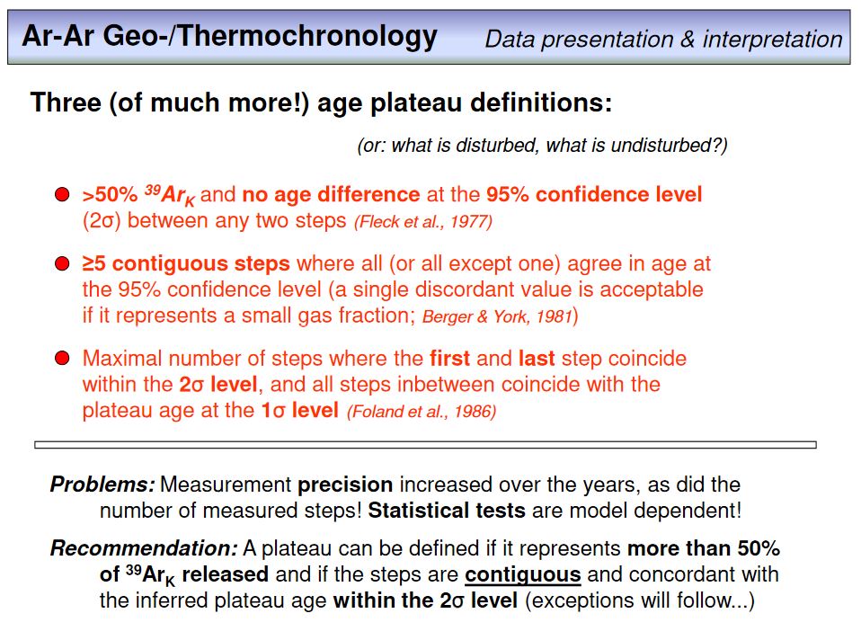 You have learned now that the Ar-Ar method provides means to test the internal consistency of a set of data used to derive a cooling age of a rock or mineral. By convention, if a sample provides a good plateau, the age derived from the plateau is considered as reliable. The question is, however, how to define a plateau? As you can see on this overhead numerous definitions have been suggested in the last decades, but a uniform and mandatory definition does not exist and the topic is still under intense debate since new generations of noble-gas mass spectrometers with a strongly improved analytical precision have been invented. To my personal opinion, for a plateau it is important to have a number of contiguous temperature steps which are identical in age within error, provide an atmospheric intercept in an inverse isochron diagram and comprise at least 30% of the 39ArK released. A problem with such a definition, and this holds for most plateau definitions, is the error of the age values. Simply speaking, following such a definition, the larger the error, the larger the likelyhood to obtain a plateau in an age spectrum diagram. In turn this means that higher measurement precisions make it sucessively more difficult to obtain plateau ages from Ar-Ar step heating experiments, and hence reducing the analytical precision would be the way to obtain as many ages as possible. This, however, is not serious and straightforward in a scientific sense. Therefore, more important than an overlap of steps within error, is to define an acceptable MSWD (which itself is a function of the individual errors) with respect to the scientific problem adressed. In other words, applied criteria need to be adopted to the scientific problem.
Overhead 60
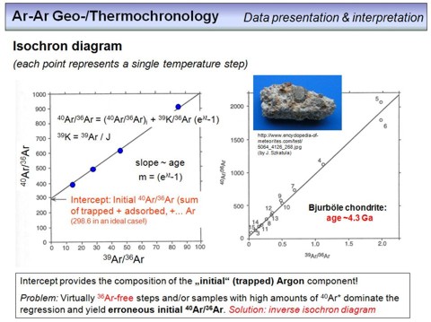 An age spectrum diagram is only one possibility to display the result of an Ar-Ar step heating experiment, and incidentally this way of presenting Ar-Ar data has the disadvantage that the age calculation for each step includes an atmospheric correction to the measured 40Ar signal. This correction is based on the atmospheric 40Ar/36Ar ratio of 298.6±0.3 (see overhead #50, it is very important to get this!). Now, as long as any argon in a sample except 40Ar* is atmospheric, this approach is fine and the resulting ages are 'correct'. If, however, all argon other than 40Ar* in a sample has a 40Ar/36Ar that deviates from the atmospheric value, the calculated ages will be wrong! Therefore, it is straightforward to label the y-axis of an age spectrum diagram as 'virtual age', and to term any 'plateau age' a model age.
Back to other ways presenting Ar-Ar data. Beyond the usage of intuitively 'easy to read' age spetra plots it is more straightforward to use isochron and inverse isochron plots that do not require the knowledge of the isotope composition of other than radiogenic argon in a sample. Two such isochron diagrams are shown on the overhead. Note that I will term any argon of a sample that is non-radiogenic as 'initial argon', although it might not be strictly 'initial', and thus terms as 'extraneous' or anything else would also be possible. The term 'initial', however, is used because the isotope composition (the 40Ar/36Ar) of the non-radiogenic argon of a sample can be determined by calculating the y-axis intercept in an isochron or inverse isochron diagram. Therefore, the term 'initial argon' is consistent with the 'initial' isotope composition knwon from other radiogenic isotope systems such as Lu-Hf, Sm-Nd or Rb-Sr.
As for any other radioisotope chronometer, the slope of a linear data array in an isochron diagram provides the age of a sample, and the y-axis intercept provides the 'initial daughter isotope ratio'. In case of Ar-Ar dating, this initial ratio is the initial 40Ar/36Ar, and if all non-radiogenic argon of a sample is atmospheric, this initial value needs to be 298.6. Only in such cases the corresponding age spectra ages are correct and therefore an isochron diagram provides control on the validness of a plateau age obtained from an age spectra plot.
The diagram on the right provides an early attempt to determine the age of the
Bjurböle meteorite.
Bjurböle is a chondritic meteorite of the low-iron (L) group and mostly consists of chondrules, with only ~10-15% matrix. As you can see, there is marked scatter in the data, so the age (~4.3 Ga) derived from the slope is rather a vague estimate than a precise radioisotope datum.
Overhead 61
The problem arising with respect to the isochron plot presented on the last overhead is the measured signal intensity of 36Ar. In an ideal case, a sample contains only value*, but no 36Ar, making the use of this plot impossible. In practice, there are samples with indeed only very little 36Ar and this causes the ratios on both axes of an isochron plot to become very large, with the consequence that the important y-axis intercept (and possibly even the slope that provides the age) becomes associated to a large uncertainty. To prevent this problem the inverse isochron plot was invented in which the 36Ar/40Ar ratio of a step is plottet versus the 39Ar/40Ar of the same step. In this case, steps with a low 36Ar signal intensity do not plot 'far off', but close to the x-axis intercept from which the age of the sample is calculated. In other words, the closer a step plots near the x-axis, the less is the 'atmospheric correction', the better. The 40Ar/36Ar ratio of the initially inherited argon component entrained by the rock or mineral during its formation is, analog to the isochron plot, provided by the y-axis intercept, hence in its inverse form.
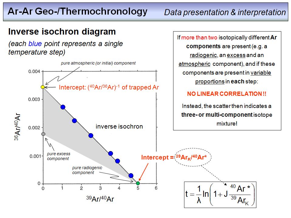 Time go one step ahead and think about the potential 'argon components' that may be present in a rock or mineral. Clearly, this is a theoretical approach as the argon that is contained in a rock or mineral will always be a mixture of five argon isotopes with corresponding ratios. But to understand inverse isochron (and isochron) diagrams, the concept of assuming different 'components' is very useful. Imagine a sample, a rock piece or mineral, that contains only two argon components, an atmospheric one (this means with a 40Ar/36Ar of 298.6 but may be any other value) and a radiogenic one. In an inverse isochron plot the atmospheric (or initial) component is free of 39Ar and thus will plot on the y-axis, in the case of an atmospheric 40Ar/36Ar at a value of 1/298.6 = 0.00335. This is the yellow point in the diagram on the overhead. By contrast, the radiogenic component is free of any 36Ar and thus will plot on the x-axis of an inverse isochron diagram, at a value determined by the age of the sample. The important point now is that different isotopes (or 'components') will be located in different positions within the lattice of a mineral, i.e. they will have different binding energies and thus will diffuse out of a mineral at different rates during heating. Therefore, any temperture step measured will be a mixture between the atmospheric (initial) and radiogenic component of the mineral. As a two-component mixing line is a straight line in an inverse isochron plot (see lecture on 'trace elements in magmatic systems'), each temperature step will plot on the line between the pure atmospheric (initial) and pure radiogenic component. These are the blue points. The position on the line depends on the ratio of atmospheric vs. radiogenic portion, and a linear regression through a number of measured steps will clearly provide the x- and y-axis intercepts and thus the 40Ar/36Ar composition of the initial component and the age of the sample.
But, what if more than two components are present, a circumstance that is often observed during measurements? The answer is fairly simple. A three component mixture in a two dimensional plot does not provide a linear correlation any more, and thus no age. Instead, any three-component mixture with varying proportions between these three components will plot within an area that is bordered by them. This is illustrated as grey field in the diagram. If a third component is added to our two-component system, for example a pure excess component (the grey point on the y-axis with an 40Ar/36Ar > 298.6), then any step that contains all three components in various portions will plot within the grey field. The same is valid for more than three components, a triangle will become a polygon with the composition of each component at its corners. Derivation of an age will be hampered!
Overhead 62
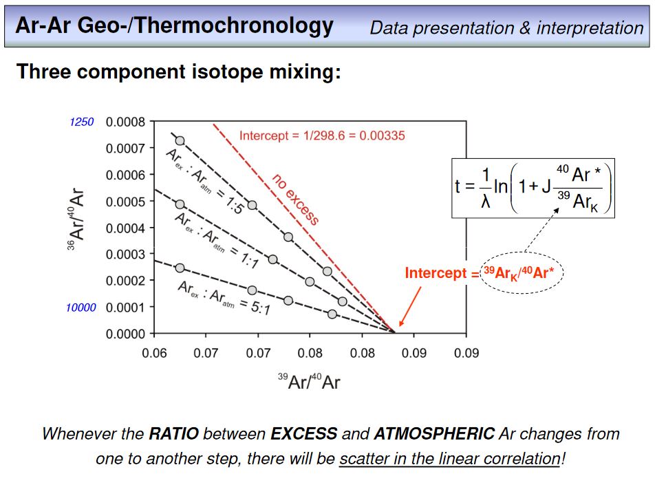 There are some restrictions with respect to what I wrote regarding a three or multiple component system, and this is the good message, with some efforts it is often possible to extract reliable ages even in more complex cases. The example shown here illustrates this for a three component system. The dashed red line is an isochron where only two components are present, an atmospheric and a radiogenic one. The y-axis intercept is the reciprocal atmospheric 40Ar/36Ar, and the age is determined by the x-axis intercept. The black dashed lines are isochrones for different but invariant mixtures of atmospheric and excess argon on the one hand, and radiogenic argon on the other. The numbers on each inverse isochron denote the invariant ratio between the excess and atmospheric component. As you can see, in cases where this ratio is constant during step wise degassing, the x-axis intercept provides a correct age, and the y-axis intercept provides the 40Ar/36Ar of the initial argon of the sample, which itself is a mixture between an atmospheric and an excess component. You might have recognized that in such cases the system behaves as a two-component system, with an initial 40Ar/36Ar that simply deviates from the atmospheric value. As you will see later, during a step heating experiment, the mixing ratio between two (or more) non-radiogenic components will nerly never be constant over the whole temperature range, but often for a few steps, which then form a linear sub-array of data that in many cases enable one to derive an age.
Overhead 63
This overhead provides a 'real dataset' obtained on an anorthoclase separate isolated from a tuff sample taken from a sedimentary-volcanic strata (Koobi Fora Formation) in the proximity of Lake Turkana in Kenya. Although there is some scatter in the datapoints, a linear regression provides an inverse isochron with an atmospheric intercept within error, and an age of 3.01 ± 0.02 Ma. The Koobi Fora Formation bordering to the east of lake Turkana in Kenya is a sedimentary-volcanic strata of considerable scientific interest and importance. Watch these two publications
(McDougall, 1985 and
Brown et al., 1985)
to find out why and provide your answer as the next
exercise.
Overhead 64
Let's see an example of a biotite separate where an inverse isochron diagram allows a more robust interpretation of a disturbed age spectrum. It is obvious that from the latter itself it is not possible to derive a reasonable age for this sample. The somehow U- or bowl-shaped spectrum, however, might be a hint on the presence of excess argon, and as you can see on the next overhead from the y-axis intercept, this biotite indeed contains an excess argon component. This causes an 'undercorrection' of the 40Ar-signal, as this correction is done by using an atmospheric 40Ar/36Ar ratio (see overhead #50), instead of a higher one that consideres also the excess component. This undercorrection, which is strongest in steps that contain lower portions of radiogenic argon, produces apparent ages that are too high. Calculating a WMA out of the steps with the lowest ages would provide a value of around 14 Ma, however, at a MSWD significantly higher than one! This MSWD would therefore reflect the disturbance caused be the presence of excess argon.
Overhead 65
This overhead shows the data of the biotite separate in an inverse isochron diagram. There is considerable scatter, but a regression provides an y-axis intercept with a reciprocal value of 375 ± 15, which clearly identifies the presence of excess argon in this biotite (likely along with an atmospheric component). The approximately linear relationship of the datapoints reveals that the ratio between atmospheric and excess argon did not change dramatically during degassing, but fluctuated slightly from one step to another. In case of this biotite, the most serious age to report would be the inverse isochron age with its associated error in the order of 1.5%. However, considering the analytical uncertainty of the individual datapoints that are not shown here, the MSWD would likely be significantly more than one.
Overheads 66 & 67
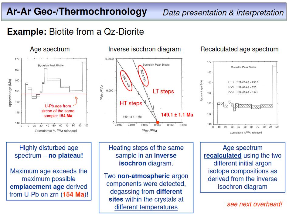 Let's move on to another illustrating example. The diagram on the left shows an age spectrum of a biotite separate out of a quartz diorite. It is obvious that the age spectrum is disturbed, and because a U-Pb zircon age from the same sample provided a crystallisation age of 154 Ma, one would expect the Ar-Ar age of the biotite to be lower.
The middle diagram shows the inverse isochron plot of the biotite. As you can see, the datapoints form two linear arrays with different slopes and thus different y-axis intercepts that reveal two different excess components in this sample (with 40Ar/36Ar of 725±125 and 1340±120). Both linear arrays, however, share the same x-axis intercept that recalculates to a cooling age of 149.1 ± 1.1 Ma. So in this sample, the low-temperature steps caused a contiguous release of an excess component with a lower 40Ar/36Ar (725) than the high-temperature steps (1340). This means that in this case it was possible to separate two different excess components by a step heating experiment, where each degassed within a different temperature range along with varying amounts of radiogenic argon of constant composition. Using the different intercept values instead of the atmospheric value to do the 'atmospheric correction' of the corresponding steps, which in this case should be termed 'correction for initial argon', the disturbed age spectrum transforms into an age spectrum with a plateau whose age is clearly the same as the inverse isochron age. This is shown in the right figure of this overhead, and enlarged and coloured on the next overhead in more detail.
Overhead 68
Some more theoretical considerations. You have seen several examples now from real samples, with more or less well defined plateaus in age spectra plots and more or less well defined linear correlations in isochron and inverse isochron
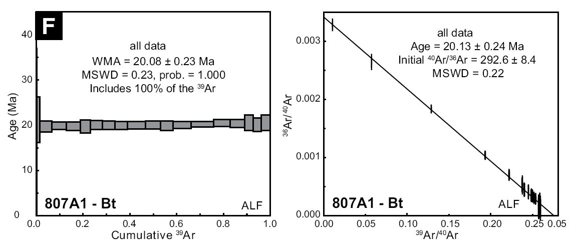 plots. But, what you haven't seen from a real sample so far is a perfect plateau, or a perfect linear correlation in an (inverse) isochron diagram. In truth such examples exist (see the figure on the right with data from a biotite separate from a sample from the Himalaya, taken from Stübner et al., 2017), but they rather make the exception than the normal case. We therefore need to ask what causes 'disturbance' in Ar-Ar datasets.
Basically, any loss or gain of argon or potassium significantly after formation or closure of a mineral will distrub the K-Ar decay system and result in disturbed age spectra and isochron plots. Such a loss or gain is typically induced by reheating, but note that movement of argon is not always out of a mineral, at appropriate partial pressures in metamorphic fluids, for example, excess argon may also diffuse into a grain. As you know, diffusion always follows the concentration gradient, and thus the direction of diffusion might be even a function of the age of a mineral, as argon becomes more over time. As different minerals in a rock contain different amounts of potassium, an argon concentration gradient will develop between different minerals over time. Such a system will therefore be in disequilibrium, and heating will cause inter-grain diffusion (reequilibration) to minimize the chemical gradients. As a consequence, the 'chronometer' in each mineral will be disturbed.
Beside thermally induced diffusion out or into a grain, any type of recrystallisation of a preexisting phase will likely disturb the K-Ar chronometer in it. This includes recrystallisation during deformation (synkinematic recrystallisation) or the formation of new phases during (low-temperature) alteration, including weathering. The net effect of any of these processes is a 'disturbed' dataset (NOT 'bad data', the data itself is usually of high quality!!), and in the following we will evaluate whether such disturbances can be figured out from the data.
Overhead 69
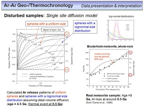 This overhead illustrates the effects of different grain sizes and/or grain size distributions on argon loss during a thermal event. The rational behind is that in step heating experiments usually not only one mineral, but several tens, hundreds or even thousands of minerals were analysed together (dating of mica, for example, with modern machines requires 1-3 mg of mineral separate, dependent on age).
The diagram on the left shows calculated 'age spectra' or 'argon release patterns' (which is essentially the same) for sherical grains with an age of 4.5 Ga that underwent reheating 500 Ma ago. Note that the data is not presented as boxes as you are used to it, but as lines, i.e. as continuum, but this makes no difference for our considerations. The black lines are argon release patterns for spherical grains with a uniform size, the numbers denote the total degree of argon loss at 500 Ma. As you can see, for a uniform grain size that corresponds to the maximum of the log-normal distribution which will be evaluated later, the original age of 4.5 Ga is only preserved in the last high-temperature steps if the total amount of argon loss is less than ~20%, and the degassing patterns are all of a convexe shape. For a
log-normal
size distribution of the analyzed split of sherical grains, the picture changes dramatically. These are the dashed curves. As you can see, for argon losses up to ~60%, the release patterns have shapes similar to what we observe for a uniform grain size, with a decreasing convexity. Note, that for the last fractions of the released argon, the age information is still very close to the original (cooling) age of 4.5 Ga, even for losses of 0.6, which strongly contrasts to what we observe for a sample with a uniform grain size.
What do you think is the reason for this? Provide your answer as the next
exercise.
The figure on the lower right shows an age spectrum (or argon release pattern) of a 'real' sample, the
Bruderheim meteorite,
a thermally overprinted (metamorphosed) ordinary chondrite of the L6 class (displayed in old fashion as points instead of boxes). The thermal overprint of the L6 class meteroites was known from textural investigations, but the question was when this overprint did occur. From the step heating experiment, which was done already more than 50 years ago, it came out that the overprint was about 500 Ma ago, whereas the initial age of the Bruderheim meteorite is 3 Ga or more.
Overhead 70
This is another example of 'disturbance' of the K-Ar clock by partial argon loss caused by a thermal event. Shown are the age spectra curves of three hornblende separates that have been isolated from three diorite samples from an intrusion with an U-Pb zircon age of 367 Ma. Importantly the three diorite samples have been taken at different distances from the contact zone towards a younger, 114 Ma old granodiorite intrusion. This granodiorite intrusion caused reheating of the preexisting diorite 114 Ma ago, clearly with decreasing temperatures with incrreasing distances from the contact zone. This is preserved in the three hornblende separates. Sample 78-420 was taken closest to the contact zone, and thus lost most of its argon during this event. Sample 78-585 was taken most far away, and thus was only little affected. Note that non of the three samples preserves the original cooling age, which is expected to be a couple of Ma less than the U-Pb zircon age, thus ~364-360 Ma, depending on the cooling rate of the diorite after intrusion. By contrast, in all three samples, the first low-temperature steps virtually provide the age of the thermal event.
Overhead 71
This example shows data of a hornblende separated from a quartz-diorite from Alaska. In this overhead you can see, how Ar-Ar data should be presented, namely two fold, first in an age spectrum plot and second in an inverse isochron plot. This sample displays a convex argon release pattern, similar to what you have seen on the previous overhead. The last high-temperature step provides a minimum initial cooling age of ~276 Ma for this sample, the first low-temperature steps provide a maximal age of metamorphism of ~140-150 Ma. Although not precise, these dates may support or argue against existing models that try to explain the geological evolution of the region of interest. Note that in this case the minimum initial cooling age of 276.0 ± 1.8 Ma was derived from the red inverse isochron in the right diagram (steps 25-28), which also indicates the presence of excess argon from its y-axis intercept with a 40Ar/36Ar of 625. Because of this, the interpretation as minimum cooling age (termed here crystallisation age) might be critical.
Overhead 72
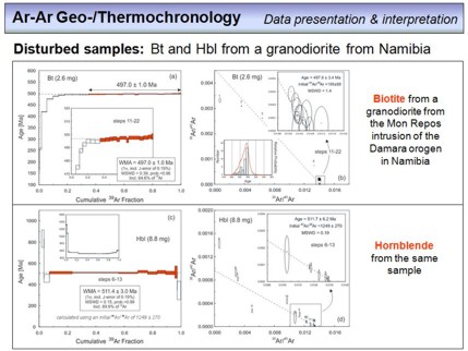 Another example of disturbed samples (phases). In the upper half of the figure data from a biotite separate is shown, in the lower half data from a hornblende separate from the same granodiorite sample. What can we see? The biotite displays partial argon loss for the first low-temperature steps, but then forms a plateau (steps 11-22) that comprises 64.6% of the released 39ArK and provides a WMA of 497.0 ± 1.0 Ma, likely the time of cooling of this biotite through ~300°C. In an inverse isochron diagram (shown in the upper right), the biotite data plot mostly very close to the x-axis. This indicates that the radiogenic component strongly dominates most of the temperture steps (which is good), with only minimal amounts of atmospheric and/or excess argon present. This is particularly the case for the plateau steps (11-22), which means that the correction for initial argon on this steps is small. The inset in this diagram shows a single grain total fusion experiment (SGTF) done on the same biotite split from this granodiorite. Here, 40 single biotite grains were dated not by step heating (SH), but by total fusion one after another, such that each grain, in principle, provides a total gas age (which equals its K-Ar age). The resulting ages were plottet in a histogram with the 'age bins' on the x-axis, and the number of ages that fall into each 'age bin' on the y-axis. From this, a probability density function was calculated, shown as red curve. The asymmetric age distribution of the SGTF ages reflects the partial argon loss that was also observed in the SH experiment, but the probability maximum is very close to the plateau age.
The dataset of the hornblende is somewhat more difficult. In the inverse isochron diagram a large scatter can be observed if all data are considered. Enlarging the lower right part, however, one can find a number of steps (6-13) that plot on a straight line, and this line forms an inverse isochron. The y-axis intercept provides a 40Ar/36Ar of 1249 ± 270. This clearly indiactes that the hornblende contains significant excess argon. The x-axis intercept provides an inverse isochron age of 511.7 ± 6.2 Ma at a MSWD of 0.19 due to the large errors on the 36Ar/40Ar values. Using the 40Ar/36Ar of the excess component (1249) to correct the data in the age spectrum for initial argon, a plateau age of 511.4 ± 3.0 Ma is observed for these steps (6-13), which comprise a total of 89.9% of the 39ArK released. You can see that in this case, by using an inverse isochron regression, it was possible to correct the data for excess argon to obtain a reasonable age.
The age difference between the biotite and hornblende is ~15 Ma, which recalculates to a linear cooling rate of ~13°C/Ma if closure temperatures of 500°C and 300°C are assumed.
Overhead 73
Rocks commonly comprise more than one mineral, and as you have seen, different minerals behave very different with respect to diffusion and thus have different closure temperatures. Therefore, it is necessary to separate pure mineral fractions out of a rock prior to irradiation and dating by the Ar-Ar method. A clean, hand picked fraction of minerals is an important pre-requisite to obtain a reliable and undisturbed Ar-Ar age, hence no guarantee.
Overhead 74
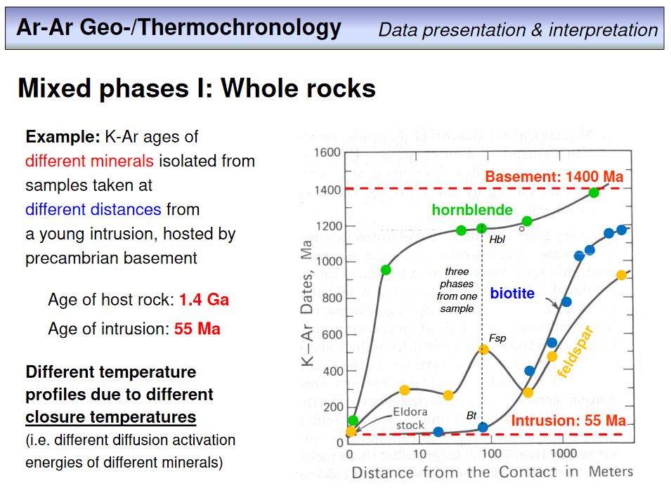 This overhead is mostly a repetition of what you have seen already, but provides another nice example that demonstrates how important it is to date only pure mineral fractions out of slowly cooled rocks.
What is shown here? The diagram displays K-Ar ages of originally 1.4 Ga old basement rocks that have been taken at increasing distances from the contact zone of a 55 Ma old intrusion. Clearly the young intrusion caused reheating of the crystalline basement, and the extent and distance of reheating is clearly visible in the K-Ar ages obtained from the different minerals that have been isolated from these samples (Ar-Ar age would provide exactly the same). As expected, at the intrusive contact, even hornblende was thermally resetted, although not completely why its age is ~120 Ma (partial resetting). K-feldspar was completely resettet and provides an estimate of the intrusion age (~50-60 Ma), biotite was not present in the sample taken directly at the contact. As you can further see, even at distances >1000 m from the contact zone, K-feldspar and biotite were strongly affected by thermal Ar-loss and therefore provide completely meaningless ages. By contrast, hornblende was not affected any more and provides the original age of the basement, i.e. ~1.4 Ga. This indicates that the temperature ~1000 m away from the contact zone was always less than ~500°C since ~1.4 Ga.
Summarizing, it is useless to say that Ar-Ar dating of the basement whole-rock samples would have been a waste of time. Information can only be gained by separating minerals prior to dating.
Overhead 75
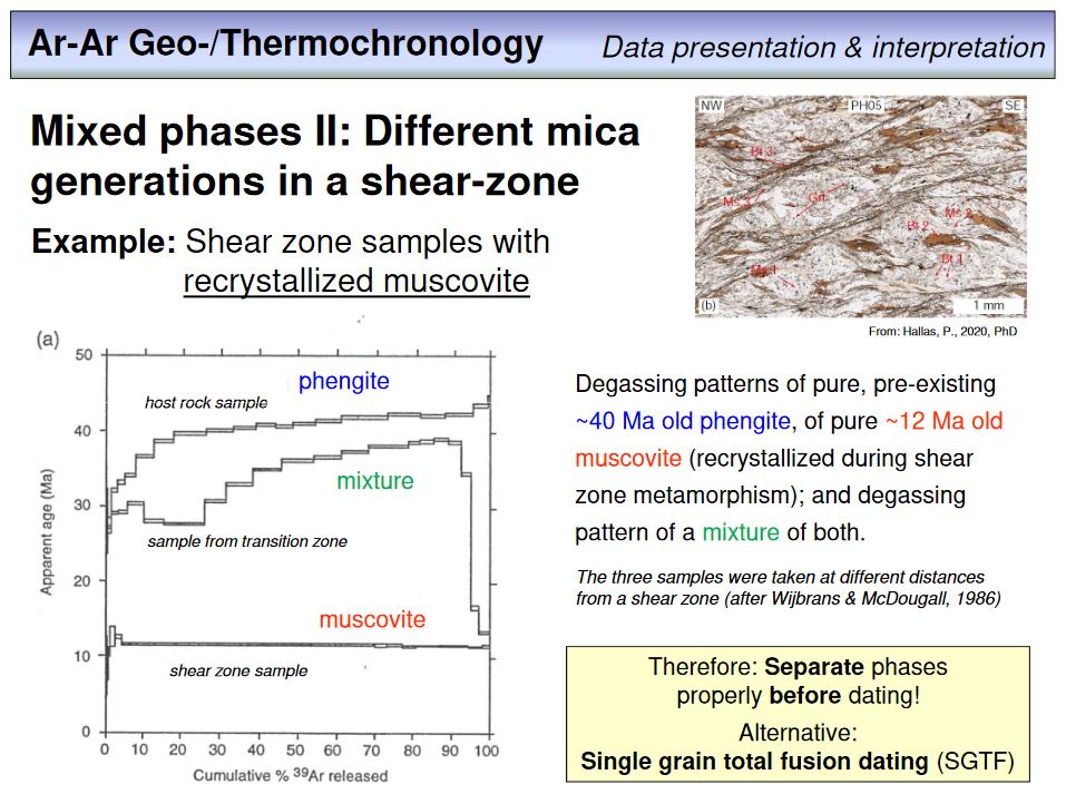 The presence of 'mixed phases' is not always so obvious as in the example of the previous overhead (where the phases have been separated anyway). In this example white mica was analysed that was separated from three samples, one directly from a shear zone, a second from a transitional zone and a third one away from the shear zone in the 40 Ma old host rock. As you can see, the 'white mica' out of the host rock is a phengite and provides an increasing age spectrum due to some argon loss, but more or less reflects the initial cooling age of the host rock. In the sample from the shear zone, the white mica is a muscovite and provides a perfect plateau with an age of 12 Ma. This is regarded as the age of shear movement that was associated to synkinematic growth of muscovite. The 'white mica' from the sample taken from the transition zone is a mixture of phengite and muscovite, and the ages provided by the step heating experiment are meaningless as they reflect mixing ages between the initial cooling age and the age of muscovite formation. Consider that in cases where such a clear association of samples to either a shear zone or a host rock is hampered, for example due to difficult outcrop situations, meaningless ages might be observed from a virtually 'clean' mineral separate (distinction of muscovite and phengite under a binocular is difficult). This, however, is fully reflected by the disturbed age spectrum.
Overhead 76
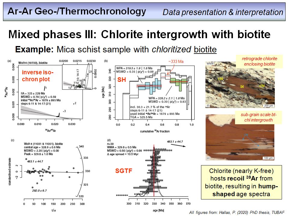 This overhead provides an example from the Erzgebirge, where a biotite separate from a mica schist was dated once by step-heating (SH) and once by single-grain total fusion (SGTF). The age spectrum of the biotite is shown in the upper middle diagram, once by using an atmospheric 40Ar/36Ar ratio for the correction of the initial argon component (grey steps), and once by using the initial 40Ar/36Ar composition as inferred (at a very large error) from the inverse isochron diagram (upper left figure). You can see that the ages of the steps markedly come down due the inferred contribution from an excess argon component (which is undercorrected if an atmospheric 40Ar/36Ar is used).
What you further can see is that the age spectrum displays an ugly 'hump', so that no distinct plateau and thus no plateau age can be defined and calculated. The common explanation for such a hump are chlorite-biotite intergrowths where the chlorite formed as retrograde phase during metamorphism from biotite. This transformation is associated to K-loss, and chlorite is nearly K-free. Therefore, this hump-shape is frequently observed in age spectra from biotite separated from retrograde overprinted metamorphic rocks. Note that even by hand-picking it is nearly impossible to separate biotite and chlorite, as these intergrowths occur on a sub-grain scale, sometimes even in unit-cell dimensions, and hence they are mostly invisible under a binocular (see the figures on the right where biotite-chlorite intercalations are shown).
The sub-micron scaled biotite-chlorite intergrowths are also the reason for the disturbance of the plateau, where the assumption is that recoil 39Ar was redistributed between biotite and chlorite during neutron irradiation. What does this mean? If the core of a 39K atom is hit by a neutron, it transforms to 39Ar and this process emitts a proton. This proton emission causes a recoil effect on the newly formed 39Ar which therefore gets dislocated within the crystal lattice by a few nm to µm. This dislocation, at a sub-micron scale, causes 39Ar from the biotite to be implanted into the chlorite. The result of this effect is a lowered 40Ar*/39ArK in parts of the chlorite, and an enlarged 40Ar*/39ArK in parts of the biotite. Note that this redistribution will be restricted to the surfaces of the phases as the dislocation length is very samll, and hence the higher the surface to volume ratio between biotite and chlorite, the stronger the recoil effect.
Back to the age spectrum. You can see that it is divided into two 'sub-plateaus'. The blue steps provide an age of 319.5±1.9 Ma, the green steps of 326.2±2.1 Ma. Inbetween we have two steps with higher ages, around 333 Ma. The interpretation is that the blue steps mostly represent chlorite degassing, with ages that are too low because of recoil 39Ar (lower than original 40Ar*/39ArK ratios). Then the two steps with the highest ages might represent primarily biotite that lost 39ArK, whereas the age are too old. Finally, the green steps are interpreted to represent predominantly undisturbed biotite, and thus carry the correct age information. A comparison with the SGTF experiment (middle and left lower figures) confirms this inference, and the WMA of all single-grain measurements provides an age of 329.5±0.5 Ma. This age is slightly higher than the 'mini-plateau age' of the green steps as no excess correction was possible for the SGTF measurements. The reason for this are 36Ar signal intensities below the detection limit of the mass-spectrometer.
Overhead 77
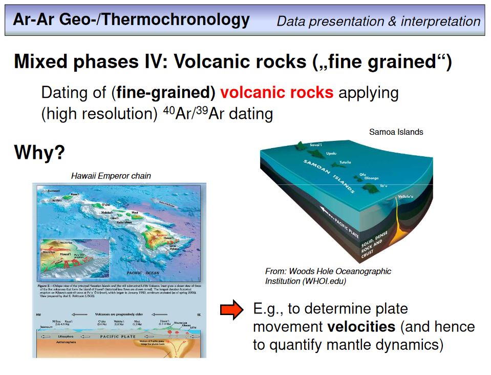 With a few exceptions we have only seen Ar-Ar data obtained on mineral separates up to here (even if these mineral separates might be 'mixed phases'). Not only separated mineral fractions can be dated, however, but also fine-grained volcanic rocks which are, by definition necessarily 'mixed phases'. This makes dating of volcanic rocks a bit critical, although different closure temperatures are irrelevant here due to very fast cooling. Note in this context that because of this Ar-Ar ages of volcanic rocks are commonly regarded as reflecting 'eruption ages'.
There are many reasons why it might be of interest to date volcanic rocks. One is the question of plate movement velocities. Watch the example on the lower left, where the movement velocity of the Pacific plate can be determined by dating the volcanic islands of the Hawaii Emperor Chain. Clearly, a prerequisite of this approach is that the Hawaiian mantle plume is regarded as having been stationary over the last 100 million years. Another example where dating of volcanic rocks might contribute to geodynamics research is the question on the movement velocities of volcanic arcs, or the question on the spatio-temporal distribution of the activity of island arc volcanoes. Speaking in a broader sense, any geodynamic approach requires the knowledge of the age of rocks, and for most mafic to intermediate volcanic rocks the Ar-Ar technique is the method of choice.
Watch these two publications
(Jicha et al., 2009 and
Sharp & Clague, 2006)
to find out how Ar-Ar dating contributes to geodynamics research and very briefly, within a few sentences, summarize in the next
exercise what you have learned.
Overhead 78
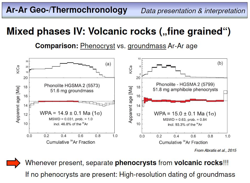 This overhead shows a comparison between dating of amphibole phenocrysts vs. groundmass fragments, both isolated from the same phonolite sample. As you can see, the groundmass provided an age of 14.9±0.1 Ma obtained from 46.8% of the 39ArK released. By contrast, the amphibole provided an age of 15.0±0.1 Ma, but from 93.3% of the 39ArK. Although both ages are identical within error the amphibole age is more robust as it comprises significantly more 39ArK, and because its MSWD is more close to one (0.63 vs. 0.031). The simple lection from this study is that whenever present, dating of K-bearing phenocrysts separated from a volcanic rock (k-feldspar, amphibole) is likely to provide more robust ages than dating of groundmass fragments. If no phenocrysts are present, apply high-resolution dating of the groundmass, where 'high-resolution' simply means measuring as many temperature steps as possible. This is to try to separate distinct argon components (compare this process to a 'distillation process').
Overhead 79
The next three overheads provide very simple explanations on what happens if either a low temperature (LT) or a high temperature (HT) step suffers 'argon loss' or does contain 'excess argon', and how this affects the inverse isochron age and y-axis intercept of a step heating experiment. Note that for reasons of simplicity only TWO steps are considered, but this concept can be applied to as many steps as required.
The left diagram on this overhead demonstrates the effect of argon loss on the LT step, and on the right you can see the effect of the presence of excess argon in the HT step. Dark red points represent undisturbed compositions, i.e. original datapoints, light red are 'disturbed points'. As you can see, argon loss shifts a temperature step to the right or upper right, and excess argon shifts a temperature step downwards to the lower left in an inverse isochron diagram. The consequence in both cases is an offsetted (disturbed) isochron with a sub-atmospheric initial 40Ar/36Ar (<298.6, the atmospheric value) and an age that is too old.
Overhead 80
The diagram on the left shows the effect of argon loss in the LT step combined with the presence of excess argon in the HT step. The result is the same as in the previous overhead. The diagram on the right shows the effect of excess argon in the LT step and an undisturbed HT step. This results in a super-atmospheric intercept value and an age that is too young (realize that, although excess is present, the age becomes too young!).
Overhead 81
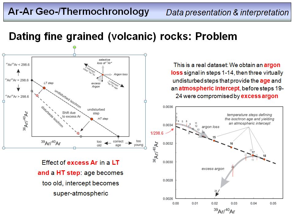 The figure on the left visualizes the effect of excess argon in both, the LT and HT step (at different proportions). In this case, the intercept becomes super-atmopsheric and the age becomes too old.
The figure on the right shows data from a real whole-rock (or groundmass) sample, namely an alkali basalt from the Central European Volcanic Province. It is obvious that this sample is 'disturbed', likely because of alteration and weathering where the formation of secondary phases (zeolithes, clay minerals) is associated with argon loss. Even intense leaching with diluted acids, including HF, and rinsing repeatedly in deionized water in an ultrasonic bath did not remove these altered phases.
The dataset suggests that the low temperature steps (1-14) reflect substantial argon loss. Steps 15 to 18 form a linear correlation, i.e. it is highly likely that these temperature steps reflect a two-component mixture between an initial and the pure radiogenic component. As the regression provides a 40Ar/36Ar intercept of 298.6, the initial argon component is pure atmosphere. The lower intercept of this correlation (the dashed line) provides the age of the sample (32.3±0.8 Ma). Steps 19 to 24 are increasingly affected by excess argon, and therefore plot successively more far away from the inferred inverse isochron.
Having these rather simple considerations in mind, you now should be able to evaluate any combination of argon loss and excess argon in a sample, even if more than two steps are considered, and to forecast the effects that will result in an inverse isochron plot.
Overhead 82
Here another example of an extremely altered whole-rock sample (basanite) that provided a fairly inconsistent dataset. As you will see, however, it was possible to extract some age information out of it.
In the inverse isochron diagram on the left one can see that nearly all low and middle temperature steps (1-16) are affected by excess argon. This is also obvious by ages up to 80 Ma in an age spectrum diagram (right). Step No. 9 is thereby the step that contained to highest amount of excess argon, and therefore provided the highest 'virtual age' (which clearly is a meaningless artefact). Steps 17 to 20 contain the age information, although at a low spreading factor (~8%), but these steps provide an atmopsheric intercept (inset in the right figure), and form a 'sub-plateau' in the age spectrum diagram that comprises 38.3% 39ArK and porivides an age of 30.6±0.3 Ma. The last two high temperature steps (21+22) again are compromised by excess argon. This sample is a good example of how even altered samples, from which no fresh material is available, can be dated by the Ar-Ar method, if a sufficiently high number of temperature steps were measured.
Overhead 83
We spent a lot of time until here with basic principles, and have undertaken a thorough discussion of data obtained during step heating experiments. But there are also some more developments and techniques to obtain Ar-Ar data, which I will very briefly describe before finishing part one of the lecture.
Overhead 84
In the last decade, a new generation of noble-gas mass spectrometers have been developed, and these instruments have improved the precision of the argon isotope data by a factor of ~5-10. The impact on step heating data is shown here for two groundmass, a sanidine and a biotite separate. The grey steps have been calculated from data obtained on a MAP 215-50 or a VG3600 noble gas mass spectrometer, both instruments developed and introduced in the 1970s and 1980s. The red steps are from data obtained on modern multi-collector noble-gas machines (ARGUS VI, Noblesse). It is obvious that the precision of data improved strongly, but consequences, for example, of this improved 'resolution' are an increasing number of samples that show overdispersion, i.e. 'geologic scatter'. Therefore, the improved technique requires also less distrubed sample material to end up with improved ages. All four samples shown here fulfill this requirement, why the ages obtained on the modern machines are up to an order of magnitude more precise (compare the dates reported for the groundmass sample in the upper left: 130±70 ka vs. 110.7±6.6 ka)!
Overhead 85
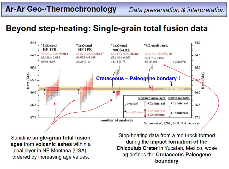 Sanidine is a common phase in evolved, SiO2-rich volcanic rocks, ashes and tuffs. It is therefore frequently used to correlate stratigraphic ages obtained on fossils with radioisotopic ages, i.e. to tack the relative time record to the absolute time record. This is possible if sedimentary strata contains concordant layers of volcanic material (ash or tuff layers, lava flows as sills, etc.). Especially for sanidine it came out that single-grain total fusion data can provide more reliable results than multi-grain step heating data, because of reasons such as temperature related isotope fractionation during step heating etc., things that are beyond the scope of this lecture.
This overhead shows sanidine SGTF data from volcanic ashes from a coal layer in NE Monatana, USA, along with SH data obtained on gass-rock formed during the impact of a meteorite that formed the Chicxulub crater in Mexico. The latter event defines the Cretaceous-Paleogene boundary and the sanidine ages, if recalculated to refined decay constants and fluence monitor ages (grey and red data), reveal that the formation of the coal layers and associated climate changes are also linked to this boundary, and thus to the meteorite impact. Note that the age spread on the y-axis of this diagram is only 3 Ma!
Overhead 86
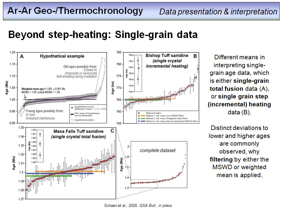 These diagrams provide (A) a synthetic dataset, where arbitrary values from normally distributed ages have been selected, and (B) single grain step heating (or incremental heating) ages from sanidine crystals, as well as (C) single grain total fusion ages also from sanidine. The observed scatter, i.e. increasing ages with steeper slopes in the front and back of the diagram, is attributed to analyical scatter on the one hand, and disturbance of the minerals on the other (excess argon, argon loss, xenocrysts, self-shielding during irradiation). Different statistical approaches exist on how to derive the best age estimate from such distributions. Two approaches, the 'low MSWD filter' and the 'weighted mean filter' (shown in orange and green) select the youngest age population for which a MSWD less than a critical value (between 1.5 and 2 dependent on the number of datapoints) can be obtained. These approaches assume that no argon loss is present even in the youngest ages, and thus seems to be critical unless this prerequisite can be confirmed by, for example, an inverse isochron atmospheric intercept of the same dataset. The third approach (in blue) searches the data subset with the largest number of ages that are normally distributed and provide a MSWD less than the critical value to calculate a mean weighted average age. The rationale behind is the assumption that the analytical uncertainty is normally distributed, but the 'geological scatter' is not. This approach is less sensitive to argon loss, and as you can see, all three approaches provide slightly different ages (insets in B and C).
Overhead 87
Last overhead, all the rage? Possibly. With the sensitivity of the new generation of noble gas mass spectrometers, in-situ dating of internal parts of minerals has become possible, although still is challenging due to technical limitations with respect to gas handling in the prep-system (blank and background problems). This overhead shows an example where an age profile through a white mica grain has been measured (see also overhead #23). This mica has recrystallized in a shear zone, and therefore is expected to provide the age of the shear zone movement. Each circle is a measurement spot, where a tiny amount of mica material has been ablated (ablation is a 'cold' process where ultrafine particles were eroded from the surface of a solid phase, i.e. comparable to 'drilling') using ultraviolett radiation (193 nm) from an excimer laser system. The numbers inside the circles are the corresponding ages of the spots, and as you can see in the age profile in the white inset, the ages increase from the left to the right margin of the grain, which might reflect prolonged growth of this white mica, possibly over a time of 4 Ma.
That's it!
www.putzfrau-agentur.de
Hinweis zum Datenschutz des verwendeten Zählers