¹⁴³
Overhead 1

Plate tectonics and magmatic processes
(accompanying explanations, © Priv.-Doz. Dr. Jörg A. Pfänder)



Textbooks you should use:
- Marjorie Wilson: Igneous Petrogenesis (Springer)
- Gunter Faure & Teresa M. Mensing: Isotopes: Principles and Applications (Wiley)
- Alan P. Dickin: Radiogenic Isotope Geology (Cambridge)
- Hugh Rollinson: Using Geochemical Data (Longman Geochemistry)

---

Note that this course requires basics from the 'Trace elements in magmatic systems' course that is held each winter term.

---

  Overhead 2
The aim of this lecture, and what you should be able to do after having gone through it. I expect that you are aware of the actualism principle, which makes the fundamental assumption to reconstruct geological processes in the past.

  Overhead 3
The tools that will be applied in this lecture are geochemical and petrological principles.

  Overhead 4
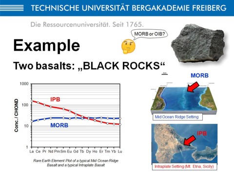Imagin a basaltic rock found in an outcrop in the forest, about 200 million years (Ma) old. The question you may adress is about the origin of this basalt, 200 Ma ago, whether in a mid-ocean ridge environment (MORB = mid ocean ridge basalt), or in a intracontinental environment (IPB = intraplate basalt)? If you grind this basalt, to make a powder of it, you can perform geochemical analyses, and then you will know the chemical composition, this means the content of most of the chemical elements of the periodic table. If you select the rare-earth elements (REE), you can plot the abundance of each REE in a chondrite-normalized REE-diagram, with a logarithmic y-axis, and this is what is shown here in the lower left. As you can see, the REE patterns of basalts from MOR and IP settings differ significantly (MORB is depleted, IPB is enriched). To summarize, chemical analyses of rocks allow us to place constraints on the origin of these rocks.

  Overhead 5
This overhead shows the different tectonic settings that will be adressed in the course of this lecture.

  Overheads 6 - 13
These overheads are all from Google Earth and show examples of different tectonic setting, with which you should be familiar already.

  Overhead 14
Let's start with the basics!

  Overhead 15
This is a very simple overview showing that we need rock powder to do chemical analyses. After crushing a representative piece of rock, e.g. by using a jaw crusher powders should be produced using an agate mill to avoid any contamination other than SiO₂, which is the most abundant species in most rocks anyway.

  Overheads 16 and 17
Once a powder is available, many different kinds of methods exist to determine elemental and isotope compositions of a rock, either from melt or powder pellets, or by digestion and solution, and subsequent chemical separation in some cases prior to analysis.

  Overheads 18 - 19
These overheads provide an example of how geochemical data tables typically look like if the results were published in a scientific journal. Major elements were usually provided as oxides in weight percent (wt%), whereas trace-elements were usually provided in parts per million (ppm). The sum of all oxides needs to be ~100%, if the loss on ignition (LOI) is included.
Overhead 19 shows the continuation of the data table. Following the trace elements, isotope compositions are given for the elements Pb, Hf, Nd and Sr. The index m denotes the measured isotope ratio, this is what we get out of our mass spectrometer, the index i denotes the initial isotope ratio that has been calculated based on the age of each sample and it parent-daughter elemental ratio (I refer here to lectures dealing with geochronology and radiogenic isotope geochemistry, and to the textbooks of Alan Dickin, Radiogenic Isotope Geology and Gunter Faure, Principles of Isotope Geology).

  Overhead 20
This overhead summarizes U and Pb concentrations along with U, Th and Pb isotope ratios measured by thermal-ionization mass spectrometry (TIMS) on a number of zircons for zircon geochronology. Each line represents data measured for a single zircon grain after dissolution and chemical separation of U-Th and Pb. The last three columns report the ages that can be calculated for each zircon from the measured data. For details see the table caption and the corresponding reference (references are given at the end of this text, and on the last overhead).

  Overhead 21
As you have seen, geochemical data related to an individual research project were reported in the articles ('papers') that emerge from these projects. However, the tremendeous increase in geochemical data over the last 20 years lead to the need of establishing database systems that make these data available to the scientific community. This overhead provides an overview over a few of the existing data repository portals. Test these links, and find out what you can find there (exercise: databases).

  Overhead 22
Let's see, what we can do with the geochemical data, either own measured one, or from a paper, or out of a database (note that using databases usually requires filtering of the data).

  Overhead 23
The first thing we can do with our chemical data is to distinguish the magmatic rocks, and to attribute them a name based on their chemical composition. The most important scheme to do so is the TAS-diagram, where TAS stands for Total-Alkali vs. Silica. For practical reasons, we have to renormalize the measured major element-oxide composition of each sample to a volatile free composition, and then we have to sum the K2O and Na2O contents (this is the total alkali value, the other alkaline elements are neglected, as they only occur in very minor abundances in most rocks). Then we can plot the TA of each sample vs. its SiO2 content. Note, that the rock-types in the grey fields were further subdivided dependent on their Na2O to K2O ratio (see table in the upper right).

  Overhead 24
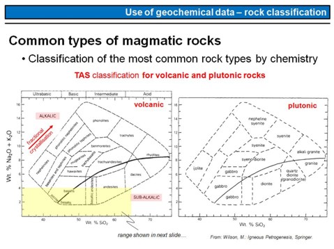An important subdivision of all the rock types in a TAS diagram into two major groups is by their total alkali-oxide content (TA: as before: TA = Na2O + K2O). This is shown by the thick black line in each diagram, the line that goes from the lower left to the middle right. All rocks below this line are termed sub-alkaline, or sub-alkalic, all rocks above this line are termed alkaline, or alkalic.
Note that fractional crystallisation of a primary, or parental mafic silicate magma, e.g. a basanite or alkali-basalt, changes the chemical composition of a magma from lower Na2O+K2O and SiO2 to higher values. This means that the chemical evolution of a magma that undergoes fractional crystallisation (and removal of crystallized phases) follows approximately the red arrow shown in the left diagram. This means, that rocks that plot more to the lower left in a TAS diagram are more primitive (or primary) than rocks that plot in the upper and upper right parts (we call them 'more evolved', or simply 'evolved' rocks).
The TAS-diagrams are the basis for the next exercise (exercise: TAS).

  Overhead 25
Have you noticed the the light yellow field in the lover left part of the left TAS diagram on the previous overhead?
This light yellow area is zoomed out and shown here, i.e. what we see here is the lower left enlarged part of the TAS-diagram. Rocks that plot within this area of a TAS diagram are further subdivided by additionally using MgO and TiO2 contents. Watch the diagram, there are names of important magmatic rocks such as komatiites, picrites, basanites, andesites or boninites. For example, boninites are rocks that typically occur in forearc-settings, where specific conditions produce partial mantle melts with high-MgO and high-SiO2, but low TiO2 contents! Note that high MgO is typically associated with low-SiO2, so boninites are in principle 'strange rocks' that require 'strange' conditions for their formation!

  Overhead 26
Further subdivisions of magmatic rocks, based on their chemical composition, can be made by considering their SiO2 vs. K2O (and/or Na2O) contents. This is shown here. Essentially we can see that the basic distinction based on the SiO2 content is maintained, with basalt (45-52 wt%), basaltic andesite (52-57 wt%), andesite (57-63 wt%), etc. (the grey vertical thick lines in the left diagram), but that the rocks in this case were further distinguished by their K-content, namely in low-K, medium-K or high-K series. Fokussing on basalts only, the terms alkalic basalts and sub-alkalic basalts are used, and the difference between both groups is defined by their Na2O at a given SiO2, as is shown in the right diagram.

  Overhead 27
Until now, we have seen what schemes are used to name rocks based on their major element oxide composition. We will now see how major and trace-element compositions can be used to decipher specific magmatic processes (for those who have participated the lecture on "Trace elements in Magmatic Systems" think about how the Ni-content of a basaltic rock can provide information about whether olivine was removed from the magma or not prior to eruption and crystallisation!).
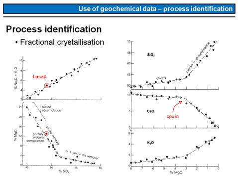The diagrams presented on this overhead show, how the composition of a magma will change if specific phases were crystallised and removed from the magma, for example by gravitational segregation.
The red point marks the composition of our starting magma, the so called parental magma that might be a primary magma or not. Starting from this composition, crystallisation of olivine and clinopyroxene will increase SiO2 along with Na2O and K2O (upper left). Contemoraneously with this, MgO in the magma will be lowered (lower left). Note that the drop in MgO is stronger if olivine crystallizes than if clinopyroxene crystallizes.
The diagrams on the right show how MgO along with SiO2, CaO and K2O will change upon olivine + clinopyroxene crystallisation (note that MgO is labelled in an inverse order, i.e. from higher contents to lower contents from left to right). Watch the evolution of the CaO in a magma, the slight drop in the beginning is due to the fact that Ca is not an element that is part of the olivine lattice. The strong drop marks the cpx in point, i.e. the moment where clinopyroxene appears on the liquidus of the system. With the beginning of cpx crystallisation, CaO will drop strongly, as Ca is an essential part of clinopyroxene (formula: (Mg,Ca,Fe)₂[Si₂O₆]).

  Overhead 28
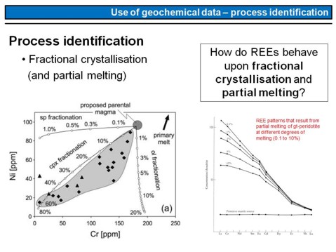This is an example of how we can use trace-elements for process identification. The left diagram shows a series of basaltic rocks and their Cr and Ni contents. To be clear, each point in this diagram represents a single sample and its associated Ni and Cr content in ppm. This means, to produce this plot, 22 samples have been taken from different outcrops in the field, and each sample has been analyzed. What we see is a broad correlation between the Cr and Ni concentration in this sample series. Note the lines with the samll circles and the numbers. These lines are fractionation trajectories, this means they show how the Cr and Ni content in a magma changes if specific phases crystallize. We have three lines, one for olivine crystallisation (ol), one for clinopyroxene crystallisation (cpx), and one for spinel crystallisation (sp). Note that the term "fractionation" here means "fractional crystallisation".
Now watch the diagram on the right. Do you know, how REE-patterns develop during successive partial melting? That is, how REE-patterns change if we increase the degree of mantle melting? This is shown here, for partial melting of a garnet peridotite with melting degrees of 0.1%, 1%, 2%, 5% and 10%. Note, that the higher the degree of melting, the lower is the slope of the REE-diagram. Can you explain, why the Lu and Yb contents are nearly invariant, that is independent of the dgree of melting, whereas La and Ce are strongly variable? And in what way do REE-patterns change for fractional crystallisation of Ol + Cpx? This is the next exercise (REE).

  Overhead 29
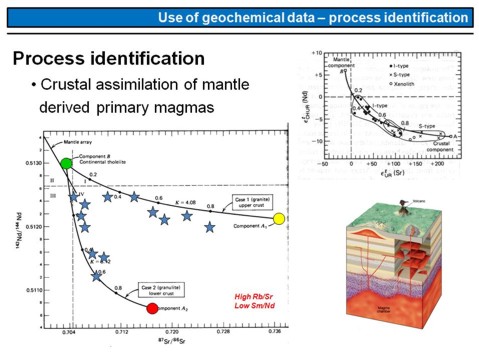If basaltic magmas that have formed within the Earth's mantle rise upwards through the continental lithosphere and crust, they may or may not interact with the continental crust (figure on the lower right). The best way to test whether a suite of basaltic rocks has assimilated continental crust is to measure its Nd, Sr, Hf and/or Pb isotope composition. An example is given here in the left diagram. Each star represents the Nd and Sr isotope composition of a basaltic rock. The datapoints build two arrays, one that connects the green point with the yellow point, this array is a mixing correlation between the primary mantle magma (green point) and upper continental crust (yellow point). The closer a datapoint, i.e. a blue star, plots to the right, the more upper crustal material has been assimilated by the basalt that is represented by this point. The same is valid for the second array that connects the green point with the red point (lower continental crust), i.e. this array represents a mixing array between the primary mantle derived basalt and lower continental crust.
What else should you learn from this diagram? You should realize that mantle derived (basaltic) magmas have radiogenic Nd-isotope compositions, that is high ¹⁴³Nd/¹⁴⁴Nd isotope ratios, but unradiogenic Sr-isotope compositions, The upper crust is intermediate in Nd, but radiogenic in Sr, and the lower continental crust is unradiogenic in Nd, and intermediate in Sr-isotope composition.
Do you know WHY the Nd-Sr isotope composition of mantle and crust are so different? If not, watch this and go through the chapters Sm-Nd dating and geochemistry of Nd-isotopes in the textbooks!
The diagram on the upper right is similar to the previous one, but here the ε-notation is used to express the Nd- and Sr-isotope composition of the samples. What we can se is a similar tend as in the larger diagram, where a mantle component mixes with a crustal component. The dots represent

  Overhead 30
Many people have tried to establish geochemical parameters that can be used to place constraints on the tectonic setting in which the corresponding rock was formed. It has turned out, however, that even such an approach is desireable, it is difficult to realize it.
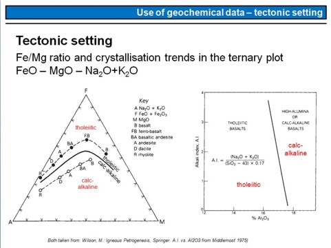
Nevertheless, this overhead is an example of how a tectonic setting affects the crystallisation differentiation of a basaltic magma. A basaltic magma that forms beneath a mid-ocean ridge (MOR; black point in the AFM diagram on the left denoted 'B') is nominally dry, i.e. water poor with usually less than ~0.5 wt% of water. Therefore, reducing chemical conditions prevail, and most of the iron in the magma will be present in its reduced form, this means as Fe²⁺. Crystallisation and removal of predominantly Mg-rich olivine (Mg,Fe)2[SiO4] will therefore cause Fe²⁺ enrichement in the magma, along with the enrichement of alkali metals (Na,K,..), until a ferrobasalt (FB; black point) and subsequently a basaltic andesite (BA), andesite (A) etc. will crystallise from the evolving magma. Such a differentiation trend is called tholeiitic trend.
By contrast, a basalt that forms in an island arc setting by fluid-induced melting of the sub-arc mantle wedge will have significantly higher water contents of several wt%. Such a magma will therefore be oxygen-rich, i.e. oxidizing conditions prevail and a significant part of the iron in the magma will be present in its oxidized form as Fe³⁺. Because of this, Fe-Ti-oxide phases such as Ti-magnetite will crystallize very early, along with olivine, and will be removed from the evolving melt. Therefore, no early stage Fe-enrichement is observed in such setting and the magma will evolve along the so called calc-alkaline trend (white points in the left diagram, from basalt (B) to dacite (D) or even rhyolite (R). Simply summarised this means, very roughly, that the Fe-content of a rock relative to its Mg- and alkali-content can be indicative whether a magmatic rock originated in a MOR- or in an island-arc setting.
The diagram on the right shows how tholeiitic and high-alumina or calc-alkaline basalts can be distinguished using their 'Alkali Index (AI)' and Al2O3-content. The AI is the molar ratio of Na2O+K2O divided by (SiO2-43)x0.17, and the subvertical line separates both basalt types.

  Overhead 31
This overhead provides an overview about different tectonic settings and their potentially characteristic magma series, whether tholeiitic, calc alkaline, or alkaline. Note that calc-alkaline series are restricted to island-arc settings, whereas tholeiites can occur in all settings, and alkaline series prevail in intra-plate settings (rifts, ocean islands). Note, however, that this is only a very rough distinction and as you will see, using the trace-element and isotope composition of rocks will provide much better constraints about their origin and evolution.

  Overhead 32
I will go into another type of tectonic discrimination schemes now, some of them are still widely used, but as you will see, most of them are not very reliable and sometimes even useless.

  Overheads 33 - 34
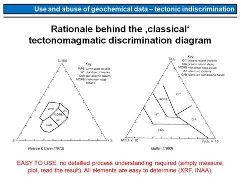What I mean are the ternary tectono-magmatic discrimination diagrams that use either major element contents, trace-element contents, or a combination of both to assign a magmatic rock to a specific tectonic setting. The rational behind these diagrams is reasonable, as on a first glance they offer the opportunity to easily assign a tectonic setting to a sample based on easy to determine parameters. However, several drawbacks emerge from this. Watch the left diagram. All tectonic settings defined here cover only about 20% of the plot area, and are very closely together. This will cause a large overlap if a series of samples is plottet, with mostly no clear result. The second issue are the rocks that might be plottet. The diagrams have been invented to assigne near-primary basalts with at least 5-6 wt% MgO to a specific tectonic setting. Therefore, these diagrams do not work for differentiated magmas and their corresponding rock types such as basaltic andesites, andesites or rhyolites, and never can be used for plutonic rocks. Why? Simply because the contents and ratios of the plottet elements are not only dependent on their mantle source composition and degree of melting, but also from the degree of fractionation and contamination. Therefore, if at all, only undifferentiated basaltic rocks that share similar degrees of melting can be plottet in such diagrams.

  Overhead 35
The invention of the afore mentioned 'discrimination diagrams' was early in the 1970s and 1980s, when only a limited number of geochemical data was available because of the limited availability of technical equipment. This changed during the late 1990s and in the 2000s, and the more high-quality geochemical data became available the more it became clear, that these 'discrimination diagrams' are only of minor value. In 2015, a somewhat provocative publication emerged that was not the first, but one of the most comprehensive that tested these discrimination diagrams and termed them 'indiscrimination diagrams'. The major conclusion that was drawn is marked here in red, and in the following I will briefly summarize the major findings.

  Overhead 36
The left diagram on this overhead shows a multi-element diagram, where the concentration of each element is denoted on the y-axis normalized to the primitiva mantle value, and as is common using a logarthmic scale. The green curve is the averaged composition of ocean island basalts (OIB), where >4000 samples have been averaged. The red curve reflects the averaged composition of island arc basalts (IAB), the blue curve is the averaged composition of mid-ocean ridge basalts (MORB). All data have been extracted from geochemical databases. As you can see, OIBs are characterised by an enriched pattern, with high La/Yb ratios. For IABs the situation is roughly the same, with a still enriched pattern but a lower La/Yb ratio. The MORB pattern is depleted, with a normalized La/Yb ratio < 1. If the averaged Zr and Y data are taken, and plottet in the discrimination diagram on the right, the OIB and MORB averages plot well within the corresponding fields, but the sole criterion is the Zr/Y variation, and the IAB point is far from the island arc basalt field. The conclusion from this simply is that a multi-element diagram provides much more power than a simple discrimination diagram. We will go into this in much more detail later.

  Overhead 37
Plotting the averaged compositions of MORB, OIB and IAB into the diagrams of Pearce & Norry (1979) and of Wood (1980), we get the following picture. Within the Pearce & Norry diagram, all points plot closely together, and IAB and MORB are nearly indistinguishable. Only OIBs plot a little more to the left due to their low HREE-contents, here reflected by the Y concentration. The Wood diagram discriminates much better, the points have significantly more spread. This is particularly because of the depleted nature of MORBs and thus the higher Hf concentration relative to Th and Ta. IABs plot more to the left if compared to OIB, at similar Hf, because of their elevated Th contents. The latter is caused (1) by the involvement of subducted sediments during IAB genesis, and (2) by the depletion of Ta and Nb in IABs. We will come back to these issues later. In summary, with respect to these three settings and averaged concentrations, the Wood diagram might best be suited to be used for discriminating between them.

  Overhead 38
These diagrams are the same as on the last overhead, but now with basalts from different tectonic settings being plottet as compositional fields instead of averaged values. The outline of each field corresponds to the 90% data contour, i.e. the 90% of the data for each setting plot within the outlined field. these fields therefore provide a good measure for the compositional variation of the respective elements. It is obvious that for individual sample suites, both diagrams will not securely work. Nearly all fields overlap each other braodly, with the exception of the OIB field that is slightly offset to the left in the left diagram. You will see, that there are much better ways to identify OIBs than these diagrams.

  Overhead 39
The same picture as before if the data are plottet in the diagrams of Pearce & Norry and of Shervais. No clear distinction is possible because of the large variation of samples from a specific tectonic setting. As for all diagrams shown until here, this picture is the same for all other discrimination diagrams that have been invented over the years.
The simple conclusion is that these diagrams might have been a good tool in the past, but that more sophisticated approaches are required if reliable information about the tectonic setting of a sample and its related magmatic evolution are desired.

  Overhead 40
What can we do? There is no unique recommendation as the appropriate approach clearly depends on the question adressed. It is important to note, however, that in an ideal case major-, trace-element- and isotope data should be integrated to place constraints on the origin of a piece of rock.
Back to the trace-element data. The best to do with them is to plot them into a multi-element concentration diagram, with primitive-mantle normalized concentrations on the logarithmic y-axis and the corresponding element on the x-axis. The order of the elements is somewhat individual, but broadly should be by 'decreasing incompatibility'. This is shown here (for details see the 'Trace elements in magmatic systems' lecture). Important features can be derived from such plots and therefore we will use them frequently during this course. Very briefly, if you watch these examples, you can see that OIBs are characterised by high enrichments of highly incompatible elements, including Nb and Ta. This is in strong contrast to island arc settings, where Nb and Ta have (in part strong) negative Nb and Ta anomalies. MORBs are less enriched to depleted, and oceanic and continental intraplate basalts are somewhere between. We will go into this in more detail later.

---

  Overhead 41
Let's start with considering individual geodynamic settings and the magmatic rock types characteristic for them. The first setting we will evaluate are mid-ocean ridges (MOR). A number of important questions can be adressed. Can you outline these questions from this overhead? Do you have own ideas on what could be important with respect to MOR settings? Provide your answer in this exercise.

  Overhead 42
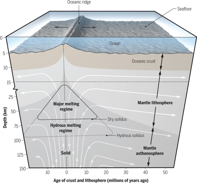
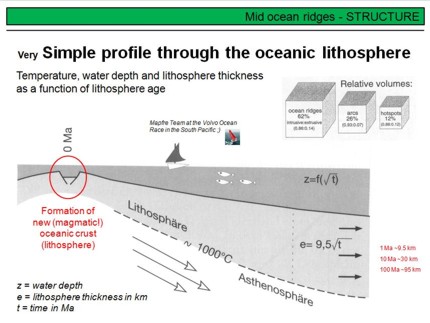This overhead shows a very simplified cross section of a MOR, and you can see, this section is not to scale but only schematic. The most important point is the fact that new magmatic oceanic crust is formed at the ridge. This mafic (basaltic) crust is hot and buoyant, but cooles down if it spreads away from the ridge axis. Note that the underlying asthenosphere also cooles to become oceanic lithospheric mantle. This is important! Cooling the rheologically weak asthenosphere at the base of the crust transforms it into more rigid lithospheric mantle. This transformation is a pure temperature effect and no material exchange is associated with it! The more the newly formed oceanic lithosphere cools, the higher becomes their density, and the deeper it sinks into the asthenosphere. Therefore, the thickness and density of the oceanic lithosphere, and thus the depth of the sea floor below sea level, is a function of time. Using the very simple formula given on the overhead, you can calculate the thickness of oceanic lithosphere from its age.

  Overhead 43
A more 'realistic' cross section across a mid-ocean ridge is shown here in the upper part of the overhead. Note the distribution of the topography with a topographic high along the ridge axis. The topography at the ridge axis depends on the spreading rate, and the latter on the magma production rate (or vice versa). Generally, at fast spreading ridges such as the East Pacific Rise (EPR) the magma production and hence the spreading rate is high, whereas at slow or ultra-slow spreading ridges, such as the Mid-Atlantic Ridge or the Gakkl Ridge, the magma production and spreading rates are low to very low.
As you know, the age distribution and hence the thickness of the oceanic lithosphere is not randomly distributed within the ocean basins, but follows a systematic that results from the spreading process itself. Therefore, the more far away from a ridge, the older an thicker is the oceanic lithosphere. A very rough age distribution is shown in the lower map. To the right on this overhead a schematic scetch of the magnetic structure of the oceanic crust is shown. As you know, the oceanic crust works like a hard disk where the magnetic polarity of the Earth's magnetic field at the time of crust formation is stored.

  Overhead 44
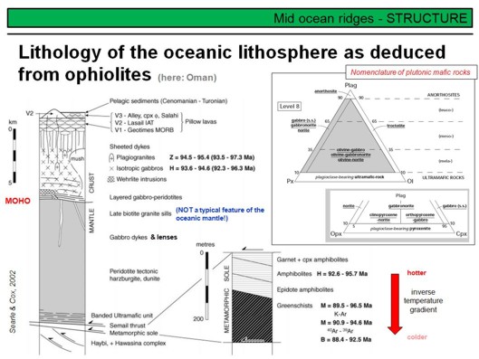This overhead shows the lithological buildup of the oceanic lithosphere as derived from ophiolites, in this case the Oman ophiolite that was formed at an oceanic spreading centre. The base, that is the former asthenospheric but now the lithospheric mantle, is made of different types of ultramafic rocks such as dunites, harzburgites, lherzolites and wehrlites (left part of the figure). In the case of the Oman ophiolite, this ultramafic section is undelain by a metamorphic sole made of amphibolites and greenschists. These amphibolites underwent high-temperature metamorphism during ophiolite obduction (see lower right part). Note the inverse temperature gradient observed in the metamorphic sole. This results from the fact that a fragment of very young and hot oceanic lithosphere overrided colder basaltic crust. The boundary between the amphibolites and the overlying ultramafic rocks is thus the thrust along which the ophiolite was obducted. In Oman, it is called the Semail thust (as the ophiolite is called the Semail ophiolite). K-Ar and Ar-Ar ages observed on amphiboles and micas from the sole are variable and scatter between 88 and 96 Ma. This is regarded as the time of obduction.
The ultramafic rocks are overlain by the gabbro unit, the boundary between both is the (ancient) MOHO. The gabbro section makes the lowest part of the oceanic crust and itself is stratified, from predominantly layered and foliated gabbros at the bottom to sucessively more isotropic and multitextured gabbros at the top. Gabbronorites, norites, wehrlites and plagiogranites occur subordinate as part of the gabbroic crustal section. Note that gabbros also occur as lenses and subordinate as dikes within the mantle part of the lithosphere. The top of the gabbro section is build by the 'rooting zone of the sheeted dikes', an area where fine grained gabbros (microgabbros) transform into sheeted dikes. The sheeted dike complex with a basaltic composition is overlain by basaltic pillow lavas intercalated with basalt lava sills and flows, all of submarine origin. The uppermost layer of the oceanic lithosphere, the ocean floor, is made of pelagic sediments (cherts, clay, red clay, pelagic carbonates dependent on depth). Concerning the lithology of the oceanic crust watch this exercise.

  Overhead 45
This overhead shows the Oman ophiolite (Semail ophiolite), as said before, a fragment of oceanic lithosphere that was obducted onto the Arabian passive continental margin ~95 Ma ago. Note the dimension of this lithosphere fragment and the distribution of the major lithologic units (peridotites, gabbros, sheeted dikes & lavas). Go to Google Earth and search for Oman. If you zoom in to the northern part of the country, you will clearly recognize the ophiolite, and you will be able to resolve the units as they are shown in this overhead. Simply search for the dark brown spots.

  Overhead 46
This overhead, on the very left, shows the seismic structure of the oceanic lithosphere, that is the distribution of the velocity of seismic p and s-waves. Note that this profile was taken "off axis", i.e. away from an active ridge segement, thus no melt can be detected by low-velocity zones (as you know, s-waves (shear waves) disappear in liquid media). As you can see, the velocity of p- and s-waves increases with depth, from ~2 and ~3 km/s up to ~4 and 7.5 km/s in MOHO regions (as you know, the MOHO is the boundary between the crust and the lithospheric part of the mantle). At the MOHO, there is a jump, and this jump indicates a change in lithology. Based on the distribution of the seismic wave velocities, the oceanic crust is subdivided into 'seismic layers. These seismic layers are termed from top to bottom 2A, 2, and 3. Each boundary between two layers corresponds to an increase in p-wave velocity.
To the right of the seismic velocity curves is a lithological profile based on ophiolite studies, where each layer is assigned a specific lithology. Note that this is only one example from many others, there are distinct differences in particular with respect to the thickness of individual lithologic layers between different ophiolites. Nevertheless, very roughly, seismic layer 2A corresponds to the pillow lavas and the upper sheeted dike complex, seismic layer 2 corresponds to the sheeted dike complex, and seismic layer 3 corresponds to the upper isotropic and lower foliated and layered gabbros. The uppermost part of the mantle, just below the MOHO, consists of ultramafic cumulates (e.g. wehrlites >>> see the text in the red box!) . Note that many of these 'ultramafic cumulates', particularly dunites, are in fact not cumulates as often thought, but residual rocks that result from orthopyroxene dissolution out of harzburgite during melt migration. The result will be a dunite where the Fo-numbers in olivine will be >0.9, i.e. a typical 'mantle value' (cumulate olivine, broadly, has Fo<0.9). See overhead #54 where dunite lenses in harzburgite are the result of melt migration by porous flow within the Earth's mantle.

  Overhead 47
Here you can see a 2-dimensional distribution of the seismic p-wave velocity across the East Pacific Rise (inset on the right). Note that the EPR is a fast-spreading ridge with a high melt production rate. In contrast to the last overhead, this seismic profile is an 'on axis profile', i.e. it crosses the ridge axis, and the goal of this investigation was to detect the zone beneath the ridge where basaltic melt is present. Note the contour lines of the seismic velocity, and the very low p-wave velocities directly beneath the ridge axis at the base of the sheeted dike complex. Generally, the lower the p-wave velocity, the higher the amount of melt present. It is important to note here that not only a 'melt lense', or a 'magma chamber' might be there (the dark red zone), but also a very large zone with 'mineral mush' (light red zone), that is a mixture of basaltic magma with a high content of minerals in it. In summary, this image visualizes the presence of basaltic melt beneath an active ridge system, and you can see that the degree of melt present increases towards the axial zone and towards the base of the sheeted dike complex, where a melt lens may be present.

  Overhead 48 (Fasten your seat belts)
We have seen a lot about the lithology of the oceanic lithosphere and the distribution of melt beneath an active ridge system until here. Now we will consider the conditions, mechanisms and processes that form the different rock types of the oceanic crust and the lithospheric mantle.
Clearly, the dominant processes are partial melting and fractional crystallisation, but whether melting occurs and to what extent is a function of mantle temperature. We therefore need to consider the distribution of heat and thus of temperature in the convecting asthenospheric mantle.
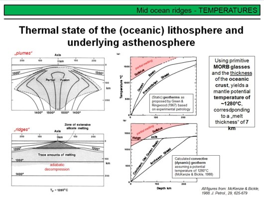
The figure on the upper left shows the proposed temperature distribution beneath a spreading ridge as suggested in the early 1980s to explain the observed magmatism at mid-ocean ridges. The black lines are isotherms, and the proposed thermal structure indicates that 'plumes' or 'jets' of hot rising asthenosphere have been proposed. Although such a hot upwelling 'jet' is suitable to explain the observed ridge topography (bathymetry), it requires high temperatures and those are inconsistent with the degree of melting and chemical composition of mid-ocean ridge basalts as deduced from experimental petrology and chemical investigations (MORB basalts were produced by roughly 10% of partial melting from garnet- or spinel peridotite and have about 10 wt% MgO, and such high temperatures would lead to much higher degrees of melting and hence to MgO contents of >15 wt% - both is not observed).
In a pioneering work, McKenzie & Bickle (1988) used the major-element composition of MORB glasses along with findings from experimental petrology and the average thickness of the oceanic crust (7 km) to estimate the temperature distribution in the upper convecting asthenospheric mantle. They found that a mantle potential temperature T_p of 1280°C produces the appropriate volume of melt to produce a 7 km thick oceanic crust, and that such a melt has ~8-10% MgO and corresponds to the required degree of melting of ~10%. This finding lead McKenzie & Bickle to suggest the upper mantle to be mostly a rather 'static' feature with a temperature structure as shown in the left lower figure.
The upper right diagram shows static geotherms for Ocean Basins and Precambrian Shields as proposed by Green & Ringwood (1967) based on experimental petrology. Static means that no mantle convection is assumed (as you know, a 'geotherm' simply describes the temperature in the Earth's interior as a function of depth, i.e. pressure). As you can see, the geotherms do not intersect the solidus of mantle peridotite, hence under static conditions the Earth's mantle would not melt! Clearly, the Earth's mantle isn't static, but convecting because of heat and thus density variations. Watch this nice video from LMU Munich, where mantle convection is modelled using supercomputers.
The diagram in the lower right shows a convective geotherm (the thick red line) with a mantle potential temperature of 1280°C as determined by McKenzie & Bickle. As convection is comparatively fast, upwelling of asthenospheric mantle peridotite is basically adiabatic, that is without loosing heat by conduction (no heat exchange of the upwelling rock with its environment). Nevertheless, as you can see, the convective geotherm has a slightly positive slope, i.e. the mantle cools slightly during upwelling. This is due to decompression, the whole process is called adiabatic decompression. Decompression means that the mantle expands by a tiny but measureable amount, i.e. its volume increases slightly, and this slight increase in volume requires energy and thus the adiabatically upwelling mantle cools. In the shown case, the mantle cools from ~1400°C at 250 km depth to ~1280°C at the surface (if melting is not considered). This cooling is only because of decompression, not because of melting! Nevertheless, as you can see, at a depth of ~45-50 km, the convective geotherm intersects the solidus of mantle peridotite, and thus will begin melting! This is the situation beneath ocean ridges.

  Overhead 49
You might have recognized that the term potential temperature was used before from time to time instead of temperature. What is the difference? The difference is that the potential temperature does not change upon compression or decompression, i.e. is the temperature (or heat) of a system corrected for the temperature change that would result from decompression in our case. In other words, the potential temperature is independent on depth. The potential temperature can be calculated from thermodynamic constants by using the uppermost formula on this overhead. The variables and some values are given in the supplementary datasheet ('handouts') that can be downloaded. As you can see, for z=0, that is at the surface as z denotes the depth in m, the exponent in the formula becomes zero, and as exp(0)=1 the potential temperature equals the physical, measurable temperature at the surface. With increasing z, i.e. depth, the temperaure increases due to compression by an amount that depends on the thermal expansion coefficient and specific heat of the mantle, whereas the potential temperature remains constant. This is the reason why the convective geotherm in the last overhead is labelled T_p = 1280°C, although the temperature changes with depth. The next exercise relates to this circumstance.
Note that a melt that rises upwards in the mantle after its formation also undelies decompression, and therefore will also cool adiabatically. The adiabatic temperature gradient of a basaltic melt is given on the overhead to be ~1 °C/km. This means that a melt that forms in 50 km depth at 1310°C will cool to 1260°C only because of decompression until it erupts at the surface (ocean floor in this case).
Note that the convective geotherm of the convecting asthenopsheric mantle (the 'adiabatic interior' in the diagrams) is a function of the viscosity of the mantle. This is illustrated in the diagrams. Watch the upper diagram. The lithosphere consists of a mechanical and a thermal boundary layer (MBL and TBL), from top to bottom. Because of the mechanical strength of the MBL, the convecting asthenosphere will never reach the surface and therefore the rising mantle will bend in a zone that is called the thermal boundary layer. This bend in material flow is expressed by a bend in the geotherm, and divides the geotherm in a convective and conductive branch. The boundary between the lithospheric and asthenospheric mantle is defined by this bend and is therefore located in the TBL. Only where the MBL and TBL are sufficiently thin, the convective geotherm will intersect the solidus, and thus melt will be produced (at T_p = 1280°C, clearly, a higher mantle potential temperature allows a thicker MBL and TBL, compare melting beneath the continents).
The two diagrams in the lower part of the overhead are enlargements of the upper diagram. It is just to demonstrate the influence of mantle viscosity on the geotherm. As you can see, a decrease in viscosity from 2 x 10¹⁷ m²/s to 4 x 10¹⁵ m²/s shifts the geotherm markedly to the left and thus the lithosphere - asthenosphere boundary from ~145 km to ~120 km depth (note that all these examples are valid for a MBL thickness of 100 km). To summarize, the amount of melt that is formed during decompression melting increases with (1) decreasing MBL thickness, (2) decreasing mantle viscosity and (3) increasing mantle potential temperature. This means that melting beneath thick continental lithosphere requires anomalously high mantle potential temperatures (>1500°C) or anomalously low solidi, i.e. the presence of fluids in the melt source region.

  Overhead 50
The dependency of the melt volume, i.e. the degree of melting, from the potential temperature of the mantle is shown on this overhead for a number of different T_p values. Under 'normal' conditions, i.e. in the source region of MOR basalts where T_p = 1280°C, melting starts at ~1.7 GPa (~45-50 km; left figure). At higher T_p, melting will start earlier (deeper), and thus the volume of melt (degree of melting) will be higher. In other words, and very important, the volume of melt that will be generated depends on the height of the melting column. The higher the temperature, the deeper (earlier) melting will start, and the thinner the lithosphere (the MBL), the shallower (later) melting will end. This means that the height of the melting column depends on T_p and the thickness of the MBL. This is graphically shown in the right diagram for different values of T_p. From this dagram we can see, for example, that for a T_p of 1480°C melting will start in ~100 km depth. Then, with ongoing upwelling and thus decompression, the degree of melting will continuously increase. If melting, for example, stops at 40 km depth (red vertical line), the amount of melt produced will be ~12 km (note that the amount of melt is expressed here as 'height' of a melt column). In other words, melting that occurs over a depth interval of ~60 km (from ~100 up to ~40 km), will produce ~12 km of melt (or a mafic crust with a thickness of ~12 km), and this corresponds to a degree of melting of 12/60 = 0.2 = 20%. To finish this a bit complicated topic, watch the following exercise.

  Overhead 51
Although not visible in the map on overhead 45, it is known from detailled mapping of lineations in the mantle peridotite units of the Oman ophiolite that small diapir like upwelling structures exist in the oceanic upper mantle. Their diameter is variable, from several hundred meters to a few kilometers. It is assumed that decompression partial melting takes place in such local upwelling zones, and not in linear features that underlie the oceanic ridges. Such a model is consistent with the existence of amagmatic transform faults that offset the magmatic parts of mid-ocean ridges. The image on the upper left shows a schematic model that visualizes how upwelling diapirs might look like. As you know, the degree of melting is a function of the depth range over which melting occurs, and this depth range depends on the mantle (potential) temperature and lithosphere thickness. The higher the temperature, the deeper the adiabatic decompression path intersects the solidus of dry peridotite and melting starts. This is shown in the diagram on the upper right. As you know, the bend of the adiabatic decompression path when it intersects the solidus is due to heat consumption during melting (fusion heat), and because of decompression. The lines denoted 0.2, 0.4, 0.6 give the degree of melting. In the diagram, the 1300°C adiabat starts melting at ~45 km depth and would produce about 20% of melt if melting would continue up to the surface. This, however, is clearly not the case as illustrated in the sketch on the lower right. The black lines are the mantle flow lines, and the red lines are the melt migration paths. Melting starts at ~60 km depth here, and the degree of melting will continuously increase from 2% up to ~15% (or even 20%). Note that melting ends exactly at the bend of each flow line, as here decompression ends!! This is the reason why the partially molten mantle beneath ridges has a triangular shape!. And also because of this, the averaged degree of melting beneath modern ocean ridges is typically in the order of 10-12%.

  Overhead 52
This overhead provides a more detailled map of a mantle diapir in the Maqusad area of the Oman ophiolite (upper right). On the left you can see how the melt delivered from such a diapir 'fuels' into preexisting oceanic crust to form locally new oceanic crust. What emerges from these detailled structural studies is that oceanic crust is not formed along straight linear features, but more 'discontinuous' by a number of more or less interfingering ridge segments, where the magmatic activity may 'jump' from time to time to other magmatic centres. This is also expressed in the striking direction of the sheeted dikes, which is not strictly in one direction, but variable with locally radial occurences.

  Overhead 53
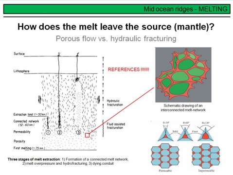Partial mantle melting occurs due to adiabatic decompression in upwelling mantle diapirs. But how is the melt distributed in the partially molten source rock, the peridotite, and how does it leave its source to form new oceanic crust? Think about petrology and ternary phase relations. Partial melting is eutectic, and thus the first melt droplets will form a grain triple junctions or binary grain boundaries. Therefore the melt will be dispersely distributed in the mantle, NOT as a huge single melt 'blob'! At some point the overall melt volume will be sufficiently high to form an interconnected melt network. This is shown on the upper right, green are the peridotite minerals, and red is the melt. The important point is that from the moment on where such a melt network forms, the melt will become mobile and able to migrate through the mantle upwards towards the ridge, driven by its lower buoyancy if compared to the solid mantle. The degree of melting required to form an interconnected melt network depends on the surface energy of a melt, and hence on its chemical composition. This is illustrated in the lower right by different wetting angles. A low wetting angle means a low viscosity and thus typically a low surface energy, such a melt will move at significantly lower melting degrees than a melt with a higher wetting angle (i.e. surface energy). Note that the wetting angle and viscosity of a magma are broady dependent on composition and temperature. A carbonatite melt, for example, has a very low wetting angle and viscosity, and will migrate in the mantle at melting degrees <1%. Basaltic melts have low SiO2 and high liquidus temperatures, and are more mobile than for example granitic melts in partially molten crustal rocks with their high SiO2 and comparatively low liquidus temperatures (~680-730°C).
Melt migration in the mantle, however, also depends on the rheology of it, and hence on the deformation rates of peridotite. At some point, the buoyancy controlled melt overpressure will exceed the tensile strength of the mantle rock such that fracturing of the mantle will occur, with a rapid melt extraction to the crust. Such different mechanisms of melt migration in the mantle, from porous flow to flow in cracks and fractures, is shown in the left figure. Note that melt extraction by hydrofracturing is likely to be discontinuous. This means that melt delivery to the crust occurs in discrete events, comparable to other magmatic vents such as volcanoes, and not continuously.

  Overhead 54
Upwards directed porous flow of basaltic magma in the mantle let the melt to cool due to decompression. Cooling, however, is not the only effect of decompression, a second important effect results from phase petrology. As you know, the stability of crystallising phases on the liquidus of a ternary system is a function of pressure (i.e. the 'area' of a phase stability field in a ternary diagram increases or decreases with a change in pressure). Basaltic magma that is in equilibrium with its host rock, i.e. with mantle peridotite, is saturated in orthopyroxene, but will become opx-undersaturated upon decompression (in other words, the stability field of opx increases with decreasing pressure). Therefore, basaltic magma that migrates upwards through mantle peridotite will dissolve orthopyroxene. If this mantle peridotite is harzburgite, i.e. peridotite depleted by previous melting events and therefore nominally cpx-free, dissolution of opx (or, chemically simply the uptake of SiO2 by the melt) will make the migrating melt more rich in SiO2 and will leave pure dunite as a residuum. This is shown in this picture taken in Wadi Abyad of the Oman ophiolite. Interconnected large dunite lenses in harzburgite are interpreted as a 3-dimensional fossile melt network. This is taken as evidence that dunits that typically occur below the MOHO to make large parts of the uppermost oceanic mantle are not of cumulate origin, but are residual mantle harzburgites formed by reactive porous melt migration. Fo-numbers >0.92 in dunite olivine support this assumption.

  Overhead 55 & 56
The image on overhead #55 shows a small scale so called 'reactive dike', i.e. a small dike or sill like ancient porous melt flow zone that is now a dunite dike in harzburgite. The dark brown surface is the typical surface colour of weathered ultramafic rocks and results from oxidized iron (rust). The brighter minerals in harzburgite are orthopyroxene.
Overhead #56 shows an ancient melt impregnation. The white dots are ancient melt droplets that now are plag-rich gabbro, the host rock is harzburgite. It is assumed that the melt overpressure was closely at the tensile strength of pridotite here, and that melt was focused in this zone towards a hydraulic fracture that outcrops to the right of this photograph, but is not visible.

  Overhead 57
Having an idea how melt forms and migrates in the mantle, we will now discuss the composition of magmas that intrude and erupt at modern mid-ocean ridges. A number of studies exist that adress this question, and I have selected two of them, the study of Presnall et al. (2002) and the comprehensive compilation of Gale et al. (2013). Most element contents are similar, and the SiO2 content of global MORB varies in the range of 47-52 wt%, i.e. is fairly constant. MgO in the Presnall et al. study is given as being between 8.4-10.9 wt%, whereas this range is markedly lower for the global compilation from Gale et al., namely between 6.2 and 0.9 wt%. The reason is that the Presnall study slectively used primitive MORB samples, i.e. such that did not underwent fractional crystallisation, whereas the Gale et al. study provides the compositional range of ALL MORB worldwide. This includes also fractionated magmas that crystallized olivine, plagioclase and clinopyroxene prior to eruption, expressed by lower contents of MgO, Al2O3 and CaO if compared to primitive MORB. Note the Na2O and K2O concentrations and the Na2O/K2O ratio that is >> 1.

  Overhead 58
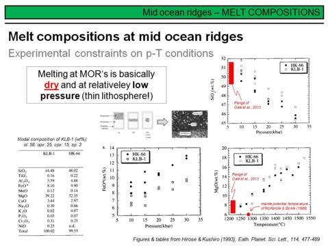How do the observed MORB compositions from 'real' samples coincide with the composition of melts from melting experiments? This is outlined here. Note that the melts erupted at mid-ocean ridges are 'accumulated fractional melts', this means that their composition is a mixture of individual melt fractions that have formed over a considerable range of pressure during decompression melting (in the melting 'column'). Even more, these 'aggregate' or 'accumulate' melts delivered from the mantle might have undergone differentiation processes such as fractional crystallisation in the crust prior to eruption. In any case, MORB samples do not provide any information about compositional variations that are relate to different melting depths (pressures). This information, however, can be obtained from melting experiments. A common peridotite that has been frequently used for partial melting experiments is KLB-1 (a peridotite xenolith from the Kilborne Hole Crater in New Mexico). Its modal mineralogy is given in the header of the table on the lower left, along with its major element composition and that of another peridotite used in experiments, HK-66. The diagrams display some of the results of these melting experiments, where melt compositions are plottet against pressure and temperature of melting. Note that these melting experiments have been conducted under dry conditions, that means without adding water to the peridotite prior to melting. As you will see later, adding fluids such as water or CO2 (in form of CaCO3) to peridotite prior to melting makes a huge difference on p and T where melting starts and also strongly affects the composition of partial mantle melts. Two major conclusions can be derived from the melting experiments. The first is that the MgO-content of a basaltic melt increases with melting temperature (and thus, at a given depth range of melting, with increasing degree of melting). This is shown on the lower right. Note that the average MgO-content of ~10.5 wt% MgO in primitive MORB as derived by Presnall at al. coincides well with the mantle potential temperature of McKenzie & Bickle, which transforms to a melting temperature in the range of 1300-1330°C in depth. The second important observation is that the SiO2-content of a basaltic melt is a function of pressure, where at higher melting pressures the SiO2-content will be lower (see the upper right figure). This is the reason, along with the degree of melting, that continental intraplate basalts are typically lower in SiO2 than MOR basalts (because they form in greater depths). To summarize some other experimental findings is subject to the next exercise.

  Overhead 59
What about the trace element composition of MOR basalts? And what conclusions can be drawn from it regarding the chemical differeniation of our planet? Consider in this context that MOR basalts sample a very large terrestrial reservoir, namely the upper part of the asthenospheric mantle!! Also note, that MORB is here considered as being representative of the oceanic crust.
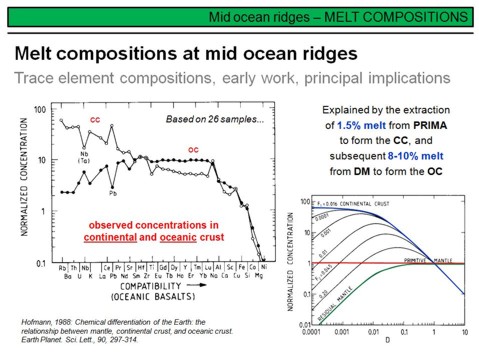
In the 1980s it became clear that MOR basalts are depleted in incompatible trace elements if compared to the primitive (primordial) mantle. By contrast, it has been recognized that samples representing the continental crust (granodiorites, granites, pelagic sediments) are enriched in incompatible trace elements. On the left figure you can see that the trace element patterns in MORB and continental crust, if normalized to the composition of the primitive mantle, are about complementary to each other. This is even valid for the Nb- and Pb anomalies and lead to the conclusion that the upper part of the Earth's mantle, from which MORB is generated, lost a considerable amount of its incompatible trace elements to the crust. Clearly, the underlying process is partial melting with an enrichement of incompatible trace elements in the melt. Based on this, the complementary chemical composition of the continental crust and Earths upper mantle was explained by crust formation through partial mantle melting. Assuming a very simple one stage model, based on melting modelling, Hofmann (1988) calculated that 1.5% of partial melting of 1/3 of the Earth's mantle with a primitive mantle like starting composition could explain the chemical composition of the continental crust. This is shown in the right figure. Such a process, in turn, would leave the upper 1/3 of the Earth's mantle (the upper mantle) such depleted, that a second melting event will produce a composition that is consistent with the observed depleted composition of present day MORB.
What does this tell us? It might feel trivial, but this simple model demonstrates that the Earth's continental crust was extracted from an originally primitive mantle to leave an upper depleted (and a possibly lower undepleted...) mantle. You will see later that the formation of the continental crust via partial mantle melting is clearly not a simple one stage process, but a complex chain of different tectono-magmatic processes that start with the formation of primitive basalt in the Earth's upper mantle, and ends with the intrusion and extrusion of granodioritic to granitic magmas in the (upper) continental crust. You will also see that the Earth's lower mantle is (mostly) not 'primitive' as one might assume from this model.

  Overhead 60
Owing to the progress in trace-element and isotope mass spectrometry, a large number of MORB analyses became available from all oceanic ridges of our planet over the last 35 years. This is shown here. Figure (A) provides the composition of global MORB, averaged from 792 samples. All elements plottet are incompatible in mantle minerals (except a few HREE in garnet), hence enriched in MORB relative to its source. The overall depleted pattern undoubtly indicates that the source of global MORB is a depleted mantle, or, in other words, the upper depleted mantle, and the reason for this was outlined in the last overhead. The overall depleted pattern displays positive Nb and Ta anomalies, and a negative Pb-anomaly. This tends to a slight enrichment (depletion) of this elements in the source relative to their neighbouring elements. Figure (B) elucidates the differences between N-MORB and global MORB, and compares them to previous estimates published earlier. Figure (C) compares the MORB data to averaged compositions of ocean island (OIB) and island arc basalts (IAB), asa well as averaged continental crust. Note that the continental crust and OIB display strongly enriched patterns contrasting MORB and IAB, and thus need to have enriched sources. But more about this later!

  Overhead 61
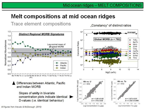The left diagram on this overhead compares averaged trace element compositions of Atlantic, Pacific and Indian MORB. Note that the concentrations are normalized to global MORB here so that this diagram shows deviations from the global MORB composition. Assuming a similar degree of melting, the Atlantic depleted mantle is therefore less depleted than the Pacific and Indian depleted mantle. There are also distinct differences between Pacific and Indian MORB, particularly with respect to the highly incompatible trace elements. These data demonstrate, little surprising, that the upper depleted mantle of the Earth is not homogeneous, but has variable degrees of depletion. Efficient mixing of the Earth's mantle through Earth's history therefore did not take place.
The diagram on the right provides a number of frequently used trace element ratios to characterize different melt source regions. As you can see, although there is a remarkable scatter (note the logarithmic y-axis) for most of the ratios, they are invariant with increasing MgO. This indicates that these ratios are largely independent from the degree of melting and crystal fractionation, and thus their values mirror the corresponding values in the magma source.
The figure on the lower right demonstrates the variation of Nb, Ta and U concentration in global MORB. Despite the fact that these concentrations vary about two to three orders of magnitude in global MORB, the linear correlation between Nb and U and Nb and Ta at a slope of ~1 indicates that Nb/U and Nb/Ta in MORB and thus in the source regions of MORB are about constant (as you have seen on the upper right figure). To conclude, ratios of highly incompatible trace elements are powerfull tools in characterising the chemical fingerprint of magma sources, as they were only little modified by partial melting or fractional crystallisation processes.

  Overhead 62
More frequently used trace element pairs of global MORB in bivariate plots and corresponding slopes. Note that for Ce-Pb there are marked deviations at lower concentrations. Note also that the overall variation for moderately incompatible trace elements such as Y and Ho is an order of magnitude less, an observation that was already clear from the multi-element concentration diagrams of the previous overheads.

  Overhead 63
Lets move from trace element compositions of mid-ocean ridge basalts to their radiogenic isotope signatures. The left diagram shows the present day Nd-Sr isotope composition of MORB from the Pacific, Atlantic and Indian ridges (for the Nd-isotope composition the ε-notation is used, see lower right for definition and also overhead #68). The data shown in these plots were taken from the GEOROC and PetDB databases that you have evaluated already. Whereas Atlantic and Pacific MORB seem to be indistinguishable, with more variation in the case of Atlantic MORB, Indian MORB seems to be, on average, slightly more radiogenic in Sr, and slightly less radiogenic in Nd. If you relate this observation to the overall abundances of trace elements as shown on overhead #61, is this what you would expect? Provide the answer as the following exercise.
The diagram on the upper right compares the Nd-Sr isotope composition of different types of ocean island basalts (OIB), and as you can see, many of them are more radiogenic in Sr and less radiogenic in Nd.

  Overhead 64
This overhead provides the lead isotope composition of mid-ocean ridge basalts, and the underlying decay schemes. The non-radiogenic reference isotope in the case of lead isotope compositions is ²⁰⁴Pb, the radiogenic isotopes are ²⁰⁶Pb from ²³⁸U, ²⁰⁷Pb from ²³⁵U and ²⁰⁸Pb from ²³²Th. So, the Pb-isotope space combines two parent isotopes from one element (U) with another element (Th) with different geochemical behaviour. It therefore provides a very powerfull tool in deciphering geochemical processes over geological time.
As you can see, no distinct differences exist, only Indian MORB seems to be very slightly enriched in ²⁰⁸Pb compared to Atlantic and Pacific MORB. This would imply a slightly higher time-integrated Th/U ratio of the Indian MORB source mantle over the Atlantic and Pacific MORB source mantle. As you will see later, Pb-isotopes are very helpful in mapping distinct mantle plume compositions as these are sampled by ocean island basalts.

  Overhead 65
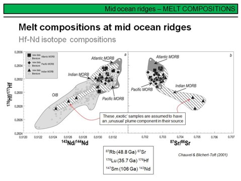More isotope systematics in MORB, here 176Hf/177Hf vs. ¹⁴³Nd/¹⁴⁴Nd. As for the Sm-Nd decay system, for the Lu-Hf decay system the daughter-isotope is more incompatible than the parent isotope during partial melting in mafic systems. Therefore, depleted reservoirs develop to radiogenic Hf isotope compositions over time, and enriched reservoirs to unradiogenic compositions (if compared to a primitive or chondritic reference). And as the fractionation of Sm and Nd, the fractionation of Lu and Hf is strongly controlled by garnet-bearing systems, even more than is the case for the Sm-Nd pair. This is the reason, for example, why garnet-bearing lithologies can be precisely dated by the Lu-Hf decay system. In general, for most lithologies, the Lu-Hf and Sm-Nd systems are strongly coupled. Decoupling, however, is indicative for selective phases and/or processes, and thus the combination of the Lu-Hf and Sm-Nd systems is a powerful tool in deciphering very specific Earth system processes such as for example the role of ultra-low degree carbonatitic melts in metasomatizing the subcontinental lithospheric mantle.
Watching the diagrams you can see that, as for Sr, Nd and Pb-isotope systematics, the Indian ocean MORB is broadly similar to Atlantic and Pacific MORB, but that a few samples extent to unradiogenic Nd-Hf values. These samples, three in this case, have correspondingly radiogenic Sr isotope compositions and are thought to reflect the presence of an enriched plume mantle component in their source.
The box in the lower part of the overhead provides, as on the overheads before, the decay systems of the plottet daughter isotopes along with the corresponding half-lifes of their parent isotopes in billion years (Ga).

  Overhead 66
This overhead summarizes a first-order explanation of the observed isotope composition of mid-ocean ridge basalts for the mentioned but also for other decay systems, and under the assumption that the evolution of the Earth's continental crust is intrinsically linked to the evolution of the upper depleted mantle. Single or multi-stage partial melting causes the formation of a depleted upper mantle (DM) and a complementary enriched continental crust (CC). Both reservoirs will develop isotope signatures corresponding to their fractionated parent to daughter element (isotope) ratios, but the most important thing here to note is time. Only if enough time elapses, DM and CC will develop the observed isotope compositions.

  Overhead 67
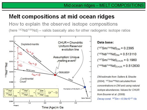This overhead illustrates a very important basic concept of radiogenic isotope systematics and in this respect is hopefully a repetition of what you have learned already. If not, here a brief explanation.
A system, this is a rock or a mineral or a melt or anything else, always becomes more radiogenic over time, never less radiogenic. Simply because radioactive decay is irrevesible and only happens in one direction! Therefore, whether something is 'radiogenic' or 'unradiogenic' rather means that something is 'more radiogenic' or 'less radiogenic'. Watch the diagram. The Earth formed from the solar nebula ~4.56 Ga ago, this is the blue point. The chemical composition of the Earth after formation is assumed to be chondritic (whatever this means!), and is termed here CHUR (chondritic uniform reservoir). Clearly this is a model composition but something we can calculate with! The CHUR and DM compositions in terms of Sm/¹⁴⁴Nd and ¹⁴³Nd/¹⁴⁴Nd are given on the right. CHUR develops with time to a more radiogenic ¹⁴³Nd/¹⁴⁴Nd isotope composition, the slope of the 'evolution line' is determined by the Sm/Nd ratio (this is equal to the ¹⁴⁷Sm/¹⁴⁴Nd which results from the present day isotope abundances of Sm and Nd). The higher the Sm/Nd, the steeper the (negative) slope of this evolution linein the diagram on the overhead. The formula given in the lower left is the formula with which the isotope evolution lines have been calculated in this diagram. The only parameters required are the present day ¹⁴³Nd/¹⁴⁴Nd of a system (rock, mineral, reservoir,...), and its Sm/Nd ratio (or its ¹⁴⁷Sm/¹⁴⁴Nd ratio) defining the slope. Having these values, any isotope composition in the past can be calculated.
Imagine what happens if our developing CHUR undergoes melting at ~2.7 Ga, that is ~1.86 Ga after Earth formation and termed 'unique melting event' on the overhead. Clearly during melting, Sm/Nd (and many other element ratios!) will fractionate, to form a low Sm/Nd melt and a high Sm/Nd residue. And because the Sm/Nd ratio changes, the slopes of the Nd isotope evpolution lines will change in a way that the melt developes to a less radiogenic Nd isotope composition over time, and the residue to a more radiogenic Nd isotope composition over time, both relative to CHUR. As you can imagine, this concept valids for all radiogenic isotope systems, and the key is always fractionation of the parent to daughter isotope ratio.

  Overhead 68
Here the equations for the Nd isotope evolution of the depleted mantle and CHUR are given, it is the same as on the previous overhead. A slight addition you can find below, it is the formula that relates any Nd isotope composition of a rock, mineral or reservoir to that of CHUR, and transforms it into a useful numer, the εNd-value. Due to this definition the εNd of CHUR is always zero, independent of time. A more radiogenic Nd isotope composition of a sample than in CHUR transforms to an εNd > 0, and vice versa. This is also illustrated in the diagram on overhead #67. To finish this brief excursus, see the following exercise.


  Overhead 69
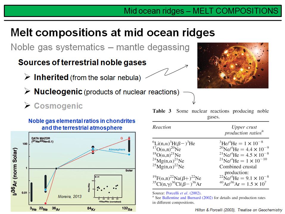Some words about noble gas systematics of our solar system and the Earth, as it will provide some interesting aspects about the interior of our planet, from data observed on MORB but also later when we will discuss the origin of ocean island basalts (OIB).
Why noble gas investigations? Foremost because noble gases are highly volatile, and therefore provide other constraints on Earth science processes than, for example, many trace elements. Furthermore, some noble gases, such as for example ⁴⁰Ar, are decay products from other elements. Noble gases were also produced as stable end products during a number of naturally occuring nuclear reactions, which occur in the atmosphere ('cosmogenic'), in rocks or minerals. A few examples of such reactions along with estimates of production ratios in the upper crust are shown in the table on the lower right. As you can see, ³He, several Ne and ³⁶Ar is continuously produced in the Earth, mostly from reactions induced by α particles and neutrons. These particles themselves were produced from spontaneous fission of U, or the decay of naturally unstable isotopes such as ⁴⁰Ar, ²³⁵U, ²³⁸U, or ²³²Th. U and Th decay emitts a lot of α particles, which then can react at low rates with target elements such as Li, O, or Mg.
The diagram on the lower left shows the abundances of several noble gas isotopes in chondrites and the Earth's atmosphere, normalized to ³⁶Ar and the respective solar ratio (this means, for example, that the ⁸⁴Kr/³⁶Ar ratio in the atmosphere and chondrites is higher than in the solar nebula). Note that the present day solar noble gas abundances are assumed to represent the primordial noble gas abundances of the solar nebula from which the sun and our planetary system developed. Note also, that the Earth (as well as chondrites) is strongly depleted in noble gases relative to the sun due to their high volatility. You can see from the figure that in carbonaceous chondrites (represented by the Q-component; red line) and the Earth's atmosphere (blue line) Ne is depleted, whereas Kr and Xe are enriched, with a strong deficit in Xe in the Earth's atmosphere compared to chondrites. Or, in other words, with respect to noble gases the Earth's atmosphere is mostly chondritic, with the exception of Xe. This suggests that some of the terrestrial ¹³²Xe still resides in the Earth's interior, i.e. our planet is obviously not completely degassed and thus is likely to contain domains with primordial material.

  Overhead 70
Table 1 provide noble gas ratios of He, Ne and Ar in the sun, the planetary system and the Earth. Note the extreme differences in ³He/⁴He and ⁴⁰Ar/³⁶Ar between the sun (primordial values) and the Earth!
Table 2 provides parent - daughter nuclide pairs for some important noble gas isotopes, along with their production yields. Most importantly, as you can see, a lot of ⁴He (α-particles) is continuously produced in the Earth's crust and mantle from the decay of U and Th. ⁴⁰Ar is also continuously produced from ⁴⁰K, whereas little ¹³⁶Xe is produced by spontaneous fission of U, Th and Pu (Plutonium). ¹²⁹Xe and is a daughter product of the decay of ¹²⁹I, but due to the short half-life of ¹²⁹I this is an extinct decay-system.
Let's focus on Helium systematics, all other systems and their applications are beyond the scope of this course. Table 1 shows that the ³He/⁴He-ratios in the sun and the Earth differ significantly, with the ratio being much lower in the Earth's atmosphere than in the sun due to the production and outgassing of ⁴He in the Earth. To have manageable numbers, the ³He/⁴He ratio of a sample, rock or reservoir is usually expresses normalized to the ³He/⁴He ratio of the atmosphere. This is expressed by R/R_A, where R denotes ratio, and A denotes atmosphere. In other words, the ³He/⁴He ratio of the sun is 326-times that of the Earth's atmosphere, i.e. the R/R_A of the sun is 326. This is important to know in the following.

  Overhead 71
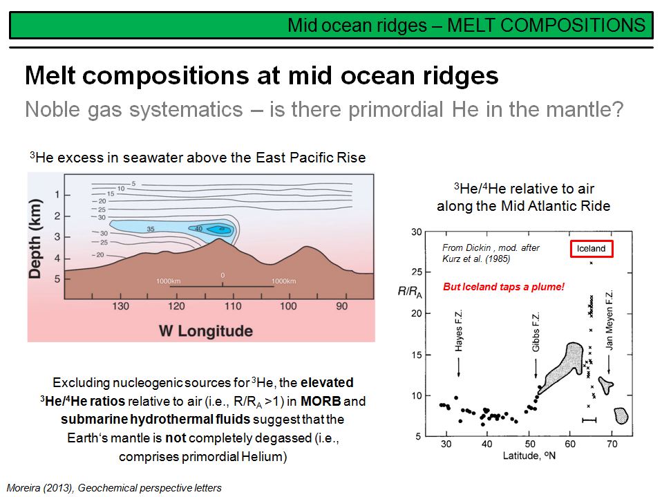There is strong thermally driven exchange between seawater and the hot oceanic crust at mid-ocean ridges as we will see later. For the moment, however, this circumstance is important as the hydrothermal circulation systems extract chemical elements from the juvenile oceanic crust, and among them is Helium. The figure on the left shows the two-dimensional distribution of ³He (expressed as R/R_A) in seawater sampled across the East Pacific Rise. It is obvious that the hydrothermal fluids sample the juvenile oceanic crust and that this crust is characterized by a ³He excess. As nucleogenic sources can be mostly ruled out, this implies that the Earths mantle is not completely degassed. It remains unclear, however, whether the upper depleted mantle itself is the source of a primordial He component, or whether a lower mantle flux continuously delivers He with a primordial component to the upper mantle and from there to the oceanic crust and atmosphere. Note in this context that the previously mentioned ¹³²Xe deficit in the atmosphere was also interpreted as being indicative for the presence of primordial material somewhere in the Earth's interior.
The figure on the right shows the He-isotopic composition of dredged MORB glases sampled along the Mid-Atlantic ridge from ~30°N to >70°N, and crossing Iceland. The Iceland samples are sub-glacial basaltic glasses. As you can see, there is an increase in excess ³He towards Iceland, with the highest values observed in Iceland samples with values exceeding 20-22 R/R_a. This strong ³He excess in some Icelandic samples is taken as indicative for the involvement of significant amounts of primordial (primitive mantle) material in the source of Icelandic basalts. Note, however, that Iceland is a setting where a deeper seated mantle plume intersects the Mid-Atlantic ridge, and hence Iceland is rather an OIB setting than a typical MORB setting. This is also the reason why Iceland is exposed subaerial.

  Overhead 72
More helium data. This overhead is somewhat like a anticipation of what will come later, as it compares different tectono-magmatic settings with respect to their He isotopic composition. It shows, however, that the ³He excess in MORB worldwide is about constant at a value of ~8 R/R_A, wheres ocean island basalts (except HIMU OIB) typically have higher degrees of ³He excess as they most likely tap deeper parts of the Earth's mantle. Continental intraplate basalts, for which a mantle plume component is often invoked during their genesis, have the broadest range in He isotope composition with values between ~20 to ~2 R/R_A. This indicates a great variety of processes and sources involved during their evolution. From a He isotope perspective we can conclude that the Earth's upper depleted mantle is fairly homogeneously degassed, whereas deeper parts of the mantle (as tapped by OIBs) are more heterogeneous with an on average higher amount of primordial material present. Low values in some continental intraplate basalts are likely to reflect a nucleogenic ⁴He component, and hence possibly the presence of assimilated continental crustal material enriched in U and Th.

  Overhead 73
Check this statement. You might have realized that the magmatic record in the oceans provides a lot of information about the origin and evolution of the Earth's mantle. With this background, we will now very briefly evaluate how the oceanic crust forms from primary basaltic magmas. Clearly, this is in principle by simple fractional crystallisation.

  Overhead 74
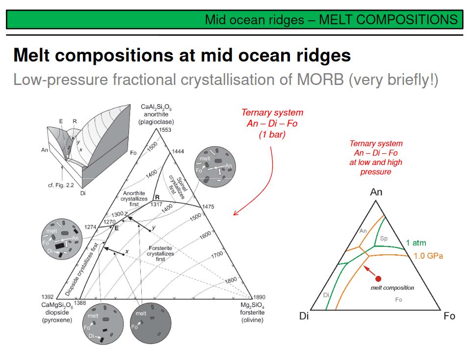This overhead is basically a repetition of what you have learned elsewhere. It exemplary shows the differentiation of a basaltic, primary olivine-normative magma at low pressure (left). The common sequence of crystallisation along the liquid line of descent is ol -> ol + plag -> ol + plag + cpx at the ternary temperature minimum (starting from the composition marked with 'y'). At high Ca/Al ratios in the melt (point 'x'), the sequence of crystallisation will be ol -> ol + cpx -> ol + cpx + plag. The same is valid at higher pressures, which lead the stability range of cpx to increase at the expense of ol and plag. This is shown on the right, where the green lines represent the phase boundaries at ~1 bar, and the red lines at 1 GPa. Note that opx is not a common liquidus phase 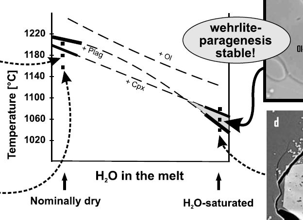in dry basaltic magmas, but may become stable at higher water activities. Water saturation of basaltic magmas also supresses the crystallisation of plagioclase and can explain the formation of wehrlites (see figure on the right, from Koepke et al., 2009), although primary MORB is nominally dry. In island arc settings, by contrast, primary basalts are commonly water-rich, and thus may crystallize Ol and Cpx to form wehrlites instead of gabbros, assisted by higher pressures.
Opx (along with amphibole) also forms as incongruent phase during water induced remelting of hot primary gabbro at mid-ocean ridges, when hydrothermal fluid circulation systems were established. This mechanism is thought to be responsible for the presence of rare norites and gabbronorites in the oceanic crust, whereas the partial melts form late stage plagiogranites.
To summarize, all igneous crustal rocks observed in the oceanic crust, i.e. gabbros, gabbronorites, norites, pyroxenites, wehrlites, hornblende-gabbros, hornblende-gabbronorites, plagiogranites, microgabbros and basalts were derived from primary basaltic magmas by fractional cristallisation. Variables that control which rock type forms are basically the pressure of crystallisation and the water content of the magma, but remelting of juvenile hot oceanic crust due to seawater infiltration also is important in the formation of opx- and amph-bearing lithologies as well as plagiogranites. Wehrlites might be either basaltic intrusions that drag large amounts of mantle olivine, or cumulate rocks that require elevated pressure or water saturation during crystallization.

  Overheads 75 & 76
As explained already in overhead 27, trends in major-element variation diagrams observed on a series of cogenetic basaltic rocks allow to deduce the sequence of crystallisation. See above for details.

  Overhead 77
It is basically the oxygen and Sr isotope composition of water bearing minerals in oceanic gabbros, such as green hornblende and pargasite, that indicates that seawater infiltration into the oceanic crust via cracks and faults reaches the base of the crust and temperatures of up to ~975°C (!). This data is shown on the lower right and although scattered, there is a clear mixing correlation from the composition of MORB mantle (that equals primary basalts) towards the composition of seawater. A model that visualizes the inferred process of establishing a thermally driven hydrothermal circulation system is shown on the upper right, and on the basis of mineral parageneses observed in the crustal section of the Oman ophiolite the authors distinguished between low-temperature (LT), high-temperature (HT) and very-high temperature (VHT) hydrothemal systems, i.e. seawater circulation within the newly formed oceanic crust occurs within different depth levels.
Beside the formation of black smokers these hydrothermal circulation systems cause intense hydratisation of the primary magmatic minerals of the oceanic crust, with the formation of new water bearing mineral assemblages that contain, for example, lawsonite, amphibole, epidote, and chlorite. Note in this context that hydratisation reactions within the crustal section and in the mantle section not necessarily take place simultaneously. We know that the mantle sections in ophiolites as well as dredged ultramafic rocks from oceanic fracture zones are typically strongly serpentinized, i.e. have taken up large amounts of seawater, but whether this process takes place at active ridges or later 'off-axis' is not fully clear.

  Overhead 78
Hydratisation and recrystallisation of primary magmatic minerals is not an isochemical process, but also causes dissolution of a number of chemical elements. The hydrothermal circulation therefore is a leaching process, and key controlling factors with respect to the solubility of minerals in hydrothermal fluids are the pH-value of the fluid and its temperature. This is shown on the right for chalcopyrite and sphalerite. Note that the y-axis is logarithmic. At a given pH the solubility of both minerals increases strongly with temperature (upper right), and at a given temperature the solubility very strongly increases with decreasing pH (lower right). Because of strongly reducing conditions within the oceanic crust, primary sulfate (SO₄^-) dissolved in seawater will be reduced to sulfide (S^2-), and the pH of the circulating fluids will be lowered successively due to the consumption of OH^- during the formation of water-bearing minerals. Enhanced sulfide concentrations, high temperatures and low pH values cause intense leaching and dissolution of metals such as Cu and Zn but also Fe in the circulating fluids, which then migrate back to the seafloor to vent as black smokers. Interaction of these 300-400°C hot hydrothermal fluids with cold seawater causes cooling and foremost a drastic increase in pH, which leads to the precipitation of metal sulfides (Fe-Cu-Zn-Mn-Fe sulfides) that may form VMS deposits (volcanogenic metal sulfide deposits). Dependent on the permeability, temperature and pH value distribution within the uppermost oceanic crust, massive sulfide deposits and stockwork mineralisation may also develop.

  Overhead 79
A summary of what we necessarily need to know about MORBs, and also the last overhead of this chapter!

  Overheads 80 & 81
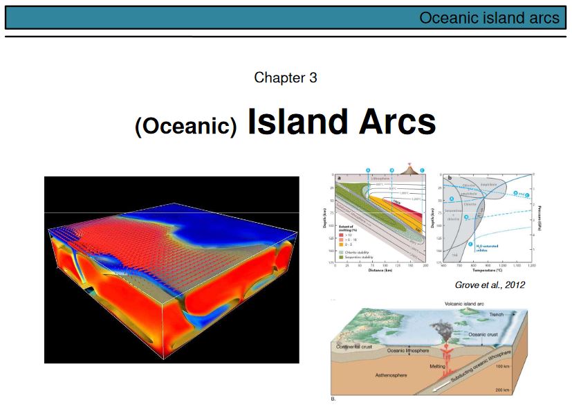With these overheads we start a new chapter, namely we will talk about island arc settings and their magmatic products in the following. Note that this chapter in part mixes up intra-oceanic and continental arcs, as primary magmas are often the same or at least very similar, but because of the differing lithosphere thicknesses in both settings the final magmatic products will be rather different.

The next overhead defines three rock types that are typical for island-arc settings, hence not the only ones. Namely adakites, which are andesitic to dacitic volcanic rocks with strongly enriched REE patterns, and strongly positive Sr-anomalies in multi-element diagrams (i.e. high Sr/Sm or Sr/Y ratios). The type locality is Adak Island in the central part of the Aleutian island arc. Then boninites, which are MgO-rich (>8 wt%) basaltic andesites or andesites, with usually very low TiO2, i.e. boninites are depleted in incompatible trace elements (La/Yb<1). Note that the combination of high-MgO contents (> 8 wt%) at SiO2 between 52 and 63 wt% is very uncommon, and never observed in a MOR setting. Usually, boninites are attributed to forearc settings, where under specific conditions a refractory mantle produces such magmas by hydrous-flux induced melting. The type locality of boninites are the Bonin Islands south of Japan. A more generalized term used to characterize island-arc related magmatic rocks is calc-alkaline, to refer to the slightly more alkali-enriched nature of most mafic to intermediate island-arc rocks relative to MOR-tholeiites.

  Overheads 82
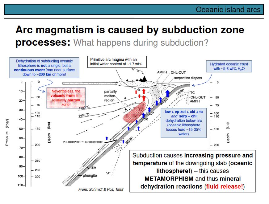This overhead shows a schematic profile through a subduction zone. Altered and hydrated oceanic lithosphere, along with relicts of pelagic sediments, becomes subducted and progradely metamorphosed. The oceanic crustal part that contains ~5-6 wt% of water becomes transferred into greenschists, amphibolites, blueschists and eclogites. The numerous hydrous minerals involved during this metamorphic process, along with the relictic primary magmatic phases (ol, cpx, plag, Fe-Ti-oxide minerals), are listet on the next overhead. Important within this context is the sucessive water release from the downgoing slab that accompanies the prograde metamorphic reactions. This water release results from breakdown reactions of hydrous minerals and is a more or less continuous process, clearly with some peaks in depth ranges, where major phase transitions occur. Overall the water, or better, the fluid phases as this is not water but rather a highly salinar supercritical liquid (see this publication for details), rises upwards into the overlying mantle wedge to react with primary mantle phases and finally to cause partial melting. These primary melts rise upwards, fractionate en-route and in lithospheric and/or crustal magma chambers forming cumulate and intrusive magmatic rocks, and finally derivatives of them become erupted as island arc volcanic series. Note that primary arc magmas contain ~1.5-2.0 wt% of water, much more than primary MOR tholeiites, which are nominally dry (<0.3 wt%).
An interesting feature is the fact that the global average depth of the surface of a subducting slab is about 100 km below the magmatic front, i.e. the active magmatic arc in present day settings (of course, varying from ~70-140 km). Also surprising is the circumstance that despite the dehydration reactions occur over a large depth range, the magmatic front is always a relatively narrow zone in recent arcs. This implies a restricted horizontal extension of the melting zone at depth.

  Overheads 83
This overhead lists a number of water bearing minerals that are common in hydrothermally altered oceanic lithosphere. Note that 'basalt' is regarded here as being representative for the whole oceanic crust, wheres peridotite is regarded as being representative for the oceanic lithospheric mantle. The numbers in parantheses denote the water content in wt%. Based on this one can see that the downgoing lithosphere carries a tremendeous amount of water from the Earth's surface to depth. Note that phengite is not a typical phase of altered oceanic crust, but becoms important where subducted pelagic sediements were metamorphosed to form mica-schists and gneises. In this respect phengite is an important carrier of potassium.

  Overheads 84
Having an idea now about the mineral assemblages that become subducted, the question arises to what extent these parageneses are stable during subduction. This overhead displays the phase relations of hydrous peridotite on the left, and of hydrous basalt on the right. Basalt represents, as usual, the basaltic and gabbroic oceanic crust. Note the tiny numbers in the rectangles, these provide the water content of the corresponding mineral assemblage!
You can see that hydrous peridotite contains between 5.9 and 6.6 wt% of water, in a sperpentine group mineral - chlorite assemblage, and that such a rock is stable up to 600°C and pressures up to 60 kbars (=6 GPa = ~180 km depth; black point with number 4 in the left diagram), before it releases water to form an ol + opx + cpx + chlorite assemblage with much less water. You can further see that following sucessive dehydration such an assemblage becomes amphibole + garnet bearing, before it starts partial melting at temperatures that exceed ~1000°C (the solidus on the right of the diagram).
Phase relations of hydrous basalt minerals at higher pT-conditions and their corresponding rock types (blueschists and eclogites), their water contents and solidus temperatures are shown in the right diagram, and you can see that hydrous basalt starts melting at much lower temperatures than hydrous peridotite, i.e. at temperatures of around 700°C at pressures around 15 kbar (~50 km). Note that such conditions are usually not reached under 'common' geothermal gradients in subduction zones (7-12°C/km).
In summary we conclude that water is continuously release from a subducting slab due to prograde metamorphism, but also that some hydrous mineral assemblages are very stable at low geothermal gradients and thus can carry water to great depths in excess of 200 km, i.e. far beyond the magmatic front of an island arc. Under 'normal' conditions, the downgoing slab will not melt.


Okay, I have to make a break, apologies ... our university admin once told us that a SCRIPT is NOT sufficient to compensate for missing lectures ... unfortunately I'm pretty sure they don't have an idea what efforts it takes to prepare a script .... so stupid ...

---

---

  Overhead 162
We have seen strong evidence that the formation of the continental crust started early in Earth's history, and that the crust forming process was not a continuous one, but occured in several pulses. When these pulses occured is somewhat model and data dependent, but most likely at ~1.2 Ga, ~1.9 Ga and between ~2.7 and 3.3 Ga. These times roughly coincide with major plate tectonic reorganizations (supercontinent cycles).
This overhead outlines the major crust forming process, or better the first step of this process, at least for Phanerozoic times (note that in the Archean crust formation might have been different). As you can see, the bulk continental crust (black circles) has the same pattern than intraoceanic island arc magmas, with a negative Nb (and Ta) and positive Pb anomaly, but with overall more enriched trace element contents. You can also see that the LILE and other highly incompatible trace elements are strongly enriched in the continental crust, but also in island arc magmas if compared to MORB. These features indicate that the formation of the continental crust requires subduction zone magmatism. In other words, the first step in the formation of the continental crust is by hydrous partial melting of an originally highly depleted and refractory mantle source, which becomes enriched in LILE and other incompatible trace elements by subduction zone dehydration priot to melting. This first-step process enriches all moderately to highly incompatible trace elements in the melt, including LILE, LREE, and Pb, but NOT Nb and Ta and NOT the HREE!

  Overhead 163
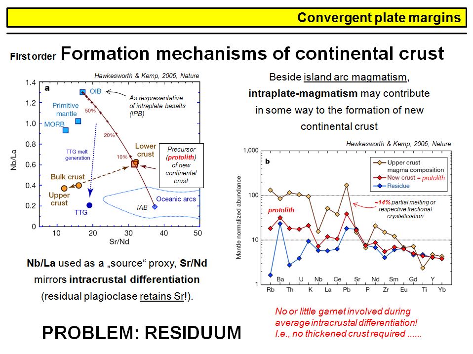Beside island arc magmatism, either in intraoceanic settings or at active continental margins, intraplate magmatism may contribute to the formation of continental crust. Hawkesworth and Kemp (2006) provided a model in which oceanic island arc magmatism (with low Nb/La but high Sr/Nd) and intraplate magmatism (with high Nb/La and low Sr/Nd) both contribute to form the mafic precursor of the bulk continental crust. Mixing proportions based on these elemental ratios suggest ~92% island arc basalt and ~8% intraplate basalt (left figure, note that Nb is very low in the first, but very high in the latter, so it is again Nb that matters). Partial remelting of this mafic precursor produces the magma from which the continental crust develops. This remelting process lowers Sr/Nd in the 'crust' as Sr is compatible in plagioclase, and because plagioclase is stable in the residue during remelting. This is an elegant model, and it explains why the Sr excess that is often observed in island arc magmas, is absent in the bulk continental crust. On the other hand, this model postulates ~14% remelting of the mafic precursor to form the continental crust, and one needs to explain where the residual 86% of this plag-rich material are.
The figure on the right outlines the trace element contents and patterns that would result from the proposed model. The red curve reflects the composition of the precursor, consisting of ~92% island arc basalt and ~8% intraplate basalt. 14% remelting of this precursor produces the continental crust (brown curve), and the residuum (blue curve). Note that Sr fractionates only very little as it is buffered by plagioclase, wheres Nd becomes strongly enriched in the crustal magma. This leads to the observed lowering in Sr/Nd during 'intracrustal differentiation' (left figure). Finally, this model does not require the presence of garnet during intracrustal differentiation to explain the HREE contents, hence no thickened continental crust, or a thick island arc. The HREE contents simply result from the composition of the mafic precursor.

  Overhead 164
This overhead summarizes and synthesizes the general crust formation model of Hawkesworth and Kemp (2006). According to this, the upper continental crust with a thickness of ~12.5 km crystallized from a melt that was produced by ~14% partial melting of a mafic precursor. The middle to lower crust, in this model, consists of a mixture of upper crust, precursor and residuum in variable proportions, with an overall thickness of ~27.5 km. This model requires a residuum layer with a thickness of ~77 km, based on mass balance considerations. This residuum is suggested to be recycled into the mantle, due to a density contrast (foundering). A problem that arises from this foundering hypothesis is the density of the residuum. This density needs to be higher than that of the mantle, which would require significant amounts of garnet to counterbalance the low density of residual plagioclase. And as we have seen, the HREE contents do not require the presence of garnet in the residuum. Nevertheless, a thick and cold mafic lower crust may form sufficient pyroxene and garnet (eclogite!) by high-grade metamorphism to enable foundering.

  Overhead 165
Plate tectonic processes may trigger such a foundering or delamination process. Significant crustal thickening caused by active continental arc magmatism and subsequent continent-continent collision, accompannied by high-grade metamorphism, may cause the required density inversion and delamination of the lower crust and lithospheric mantle. This is shown here. In any case, downsagging and separating cold lithospheric mantle and lower mafic crust will produce a 'gap' that needs to be filled, which is by more buoyant asthenospheric mantle. Delamination and the asthenospheric slipstream will (1) cause intense uplift of the remaining lithosphere in the corresponding region, and (2) post-orogenic magmatism, if the asthenospheric slipstream has an upwards tending component and if the potential temperature of the asthenosphere is sifficiently high. If no direct asthenospheric melting is possible, the asthenospheric heat may nevertheless be sufficient to trigger lower crustal remelting. In nature, most likely both processes will occur contemporaneously, and the heat of the mafic magmas will trigger partial remelting of the lower to middle crust. Note that in orogenic regions, the spatial arrangement and age distribution of post-magmatic (mafic) magmatism provides a tool to decipher the dynamics of the underlying delamination process (whether prograding into one direction as in the upper figure or randomly distributed in 'droplets' like in the lower figure).

  Overhead 166
This overhead provides an alternativ model to explain the evolution of juvenile continental crust from mafic magmas. The key process here is high-pressure fractionation of primary magmas at the base of the arc crust to form ultramafic cumulates. Solidus phases at high pressure are mostly olivine and clinopyroxene, plus some Fe-(Ti)-oxides such as spinel and/or magnetite depending on the water content and thus the oxygen fugacity of the primary magma. These ultramafic cumulates will thus be predominantly dunites (ol) and wehrlites (ol+cpx). The derivative magmas undergo further fractional crystallisation, likely at higher crustal levels, such that Al-rich phases such as garnet (higher pressure) or plagioclase (lower pressure) will crystallize along with pyroxene to form garnet-pyroxenites or gabbroic rocks. Potential remelting of such rocks will produce more evolved intermediate magmas that will crystallize diorites and granodiorites in mid-crustal levels. Clearly this is a very simplified model, but it demonstrates that a sequence of magmatic processes is required to explain the evolution of juvenile continental crust.

  Overhead 167
Formation mechanisms for juvenile continental crust clearly depend on the thickness of the island arc system, which in turn depends on the age of the arc and its growth rate (maturity of an arc system). The outlined model was developed based on the fractionation of specific trace elements (Nb and Ta), and therefore requires the presence of rutile and garnet as magmatic liquidus phases. Therefore, the outline scenario requires a thick lithosphere, this is an active continental margin. Due to cooling the density of the lower ultramafic crust of such a system will increase over time, leading to a density inversion and as in the model of Hawkesworth and Kemp (2006) to lower crustal delamination. Such a delamination process is a recycling process as is subduction, and it is debated whether it contributes to the source of OIB magmatism as well. In any case, to account for the andesitic composition of the bulk continental crust, the removal of the ultramafic-mafic lowermost parts is necessary, and therefore delamination or foundering is a likely process. As mentioned before, such a process requires rapid uplift of the remaining lithosphere and likely contemporaneous magmatic activity due to slipstreaming hot asthenosphere.

  Overhead 168
Having outlined some principle problems and models associated to the formation of juvenile continental crust, let's move ahead and ask about potential magmatic processes that are responsible for crustal internal differentiation. Such crust internal differentiation is an important process that explains the occurrence of more evolved, i.e. more silicic rocks such as granites and derivatives of them, e.g. pegmatites. Such processes are also of great importance with respect to the formation of deposits of critical raw materials such as magmatic tin, tungsten or lithium mineralizations.
Before going to the magmatic details, let's elucidate how we can decipher whether a magmatic felsic rock, e.g. a granodiorite or granite, is a juvenile or a reworked piece of continental crust.

---

www.stromanbieter.center
Hinweis zum Datenschutz des verwendeten Zählers